DGLD: Domain-Gated Latent Diffusion for the Discovery of Novel Energetic Materials

1. Introduction

Energetic-materials performance gains translate directly into reduced propellant mass, smaller warheads, and more efficient civilian gas-generators, yet the canonical anchors of the field (HMX and CL-20) were developed decades ago and no new HMX-class compound has been disclosed in fifteen years. The space of synthesisable CHNO small molecules with the right balance of crystal density, oxygen balance, heat of formation, and detonation kinetics is vast, but traditional discovery explores it slowly. Computational methods offer acceleration, yet each existing family has a fundamental limitation: empirical formulas (Kamlet–Jacobs [12]) are regime-limited; discriminative surrogates [15][16] score candidates but do not propose them; generative language models trained on energetic corpora memorise training data; and standard guidance methods [14] fail silently when the generative trajectory is as short as molecular generation requires. Compounding these challenges, the labelled corpus is tier-stratified: of ~66 k labelled rows only ~3 k come from experiment or DFT, with the rest from empirical formulas and 3D-CNN surrogates of sharply lower reliability.

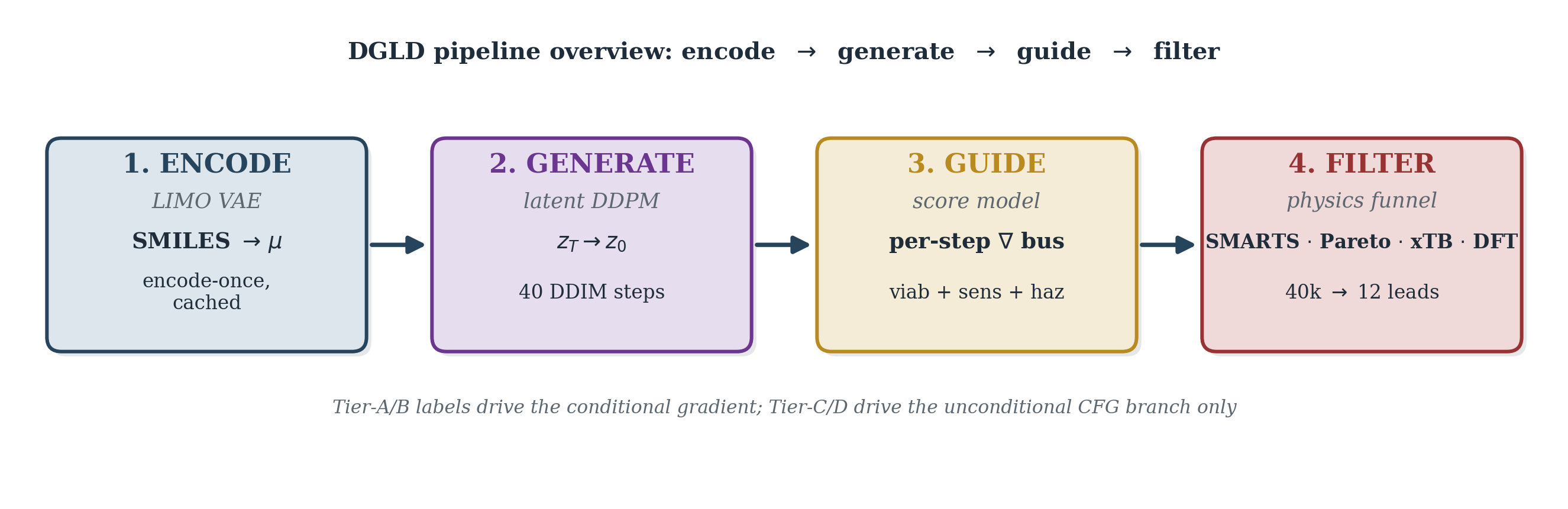
We introduce Domain-Gated Latent Diffusion (DGLD). At training time, a four-tier label-trust hierarchy gates which examples drive the conditional gradient (experimental and DFT labels) and which train only the unconditional prior (Kamlet–Jacobs and surrogate labels), preventing miscalibrated data from corrupting the generation signal. At sample time, a multi-task score model with six property and safety heads injects per-step steering into the diffusion trajectory; each head acts as an independent on/off switch without retraining the backbone. Decoded candidates pass through a four-stage validation funnel: a SMARTS chemistry gate, a Pareto reranker, semi-empirical GFN2-xTB triage, and full DFT audit (B3LYP/6-31G(d) + \(\omega\)B97X-D3BJ/def2-TZVP).

DGLD yields 12 DFT-confirmed novel leads; the headline compound, trinitro-1,2-isoxazole (L1), reaches \(\rho_{\text{cal}} = 2.09\) g/cm³ and \(D_{\text{K-J,cal}} = 8.25\) km/s, placing it within the HMX/CL-20 performance band at max-Tanimoto 0.27 to our 65 980-row labelled corpus (§5.2). DGLD behaves as a productive-quadrant generator: it samples molecules that are simultaneously novel relative to the labelled master and competitive with the HMX/CL-20 reference class on predicted detonation performance. Across three strong baselines, DGLD is the only method with consistent novel productive-quadrant coverage (simultaneously novel and on-target for performance): SMILES-LSTM memorises 18.3% of outputs exactly; SELFIES-GA returns 74% corpus rediscoveries and its best novel candidate collapses from \(D_{\text{surrogate}} = 9.73\) to \(D_{\text{DFT}} = 6.28\) km/s under DFT audit (a 3.5 km/s surrogate artefact); REINVENT 4 generates novel high-N heterocycles but peaks at \(D = 9.02\) km/s. A second lead, E1 (4-nitro-1,2,3,5-oxatriazole), reaches \(D_{\text{K-J,cal}} = 9.00\) km/s from a chemically distinct scaffold family, pending thermal stability confirmation and an oxatriazole-class DFT anchor (§6). The tier-gating recipe is domain-agnostic; only the validation funnel changes per application.

Note on Fig 1. Hz-C2 top-1 surrogate values (3D-CNN scale): \(D\) = 9.39 km/s, \(P\) = 38.7 GPa, within 5% of the strict targets. On the 6-anchor-calibrated K-J scale L1 reaches \(D_{\text{K-J,cal}}\) = 8.25 km/s and \(P_{\text{K-J,cal}}\) = 32.9 GPa, slightly below the strict thresholds but in the HMX-class band by anchor-relative ranking.

1. A tier-gated training recipe for sparse-label molecular generation. A four-tier label-trust hierarchy gates which examples drive the conditional gradient (experimental and DFT labels) and which train only the unconditional prior (Kamlet–Jacobs and surrogate labels), preventing low-confidence data from corrupting the targeted generation signal. The recipe is domain-agnostic; only the validation funnel changes per application.
2. A multi-task score model with selectable sample-time steering. Six heads share a single trunk trained jointly over viability, sensitivity, hazard, performance, and two synthesis-complexity signals. At sample time, three heads supply per-step gradient steering on the latent; per-head scales act as on/off switches over chemistry classes without retraining the diffusion backbone.
3. Self-distillation refinement of the viability head. The viability head is refined by mining the model's own false-positive outputs as hard negatives against a chemist-defined held-out probe; the production budget-918 checkpoint is round 2 of self-distillation (round 0 = score-model trained on corpus only with Random-Forest-derived viability labels and 0 hard negatives, round 1 = corpus + 137 mined hard negatives, round 2 = corpus + 918 cumulative hard negatives + aromatic-heterocycle boost), closing the gap between the Random Forest teacher's class boundary and the latent regions the sampler actually inhabits.
4. Pool-fusion sampling for scaffold diversity. Independent end-to-end sampling lanes (differentiated by denoiser checkpoint, conditioning targets, and guidance configuration) are unioned and deduplicated post-decode, making each axis an orthogonal diversity lever without increasing per-lane compute.
5. DFT-validated novel HMX-class candidates. Twelve chem-pass leads are confirmed as true local minima under B3LYP/6-31G(d) and calibrated against six reference compounds under \(\omega\)B97X-D3BJ/def2-TZVP. Lead L1 (trinitro-1,2-isoxazole) is absent from PubChem and the 65 980-row labelled master (max-Tanimoto 0.27); DFT-calibrated: \(\rho_{\text{cal}} = 2.09\) g/cm³, \(D_{\text{K-J,cal}} = 8.25\) km/s; 3D-CNN surrogate: \(D = 9.56\) km/s (see §5.3 for K-J relative-ranking basis). E1 (1,2,3,5-oxatriazole family, \(D_{\text{K-J,cal}} = 9.00\) km/s) is a further lead from a chemically distinct family, pending addition of an oxatriazole-class DFT anchor (§6); the extension set spans eight Bemis–Murcko scaffolds across six chemotype families.

2. Related work

DGLD sits at the intersection of three lines of work: molecular generative modelling, diffusion models with classifier-style guidance, and property prediction for energetic materials. The central contribution being positioned is property-targeted molecular generation under tier-stratified labels, with end-to-end first-principles audit (DFT) on energetic chemistry. The literature reviewed below either supplies a building block we adopt (LIMO encoder, classifier-free guidance, FiLM conditioning, GFN2-xTB and PySCF for validation), defines a baseline we compare against (MolMIM, MOSES-style benchmarks), or stakes out a neighbouring problem domain (3D pocket-conditioned diffusion, drug-like generative benchmarking) whose techniques we deliberately do not transplant into the energetic-materials regime. We close the section by stating explicitly which gap DGLD fills.

2.1 Molecular generative models

VAE-based molecular generators learn a continuous latent over SMILES, SELFIES, or molecular graphs and navigate it for property optimisation. Gómez-Bombarelli et al. [gomez2018] introduced the encoder/decoder recipe over SMILES; the Junction-Tree VAE of Jin, Barzilay and Jaakkola [jin2018] moved the latent up to fragment graphs to guarantee chemical validity; CDDD [winter2019] learned the latent by translating between equivalent string representations and showed that the resulting descriptors transfer to property prediction; Mol-CycleGAN [maziarka2020] reframed property optimisation as image-to-image translation between molecule sets. SELFIES [krenn2020] replaced SMILES with a syntactically robust string representation in which every token sequence decodes to a valid graph, and is the representation we adopt at the encoder boundary.

Two more recent latent generators are particularly relevant to DGLD. LIMO [eckmann2022] couples an MLP-VAE over SELFIES with a non-autoregressive decoder, factoring decoding through a per-position categorical so that gradient-based latent optimisation does not have to differentiate through autoregressive sampling; LIMO is the encoder we fine-tune. MolMIM [reidenbach2023] trains a Perceiver-encoder [jaegle2021] mutual-information VAE on billion-scale SMILES and provides a strong no-diffusion baseline against which our latent-diffusion prior is compared.

Language-modelling approaches treat SMILES directly as a string. REINVENT [olivecrona2017] trained a recurrent generator on SMILES and biased it toward design objectives via reinforcement learning; Loeffler et al. [loeffler2024] describe REINVENT 4, the modern evolution that integrates multiple generator architectures (de novo RNN, scaffold decoration, fragment linking, Mol2Mol transformer) within a unified staged RL/CL framework with a plugin scoring subsystem, and is used here as an RL-based comparative baseline. REINVENT 4 biases generation via a policy-gradient reward signal over a pretrained prior; DGLD instead learns a conditional prior through latent diffusion, separating prior learning (training) from property steering (guidance), and requires no RL reward engineering at generation time. Several REINVENT 4 mechanisms are inspirationally relevant: the diversity filter (Murcko scaffold bucketing) is analogous to our Tanimoto novelty window; staged learning mirrors our guidance-weight annealing schedule. ChemTS [yang2017] combined an RNN prior with Monte-Carlo tree search; MolGPT [bagal2022] applied a GPT-style decoder with property tokens prepended for control. MoLFormer-XL [ross2022] and Chemformer [irwin2022] showed that BERT/T5-style pretraining on hundreds of millions of SMILES yields representations that transfer cleanly to property-prediction tasks. The flow-network approach of Bengio et al. [bengio2021] reformulates non-iterative diverse candidate generation as flow matching over an implicit reward landscape and is conceptually closer to our guided sampling than to autoregressive language modelling. On the graph side, DiGress [vignac2023] performs discrete denoising diffusion directly on molecular graphs, achieving exact validity at the cost of having to re-introduce property conditioning via a separate guidance term.

2.2 Diffusion models and classifier guidance

Denoising diffusion probabilistic models [ho2020] and the score-based formulation of Song and Ermon [song2019], later unified through a stochastic-differential-equation perspective [song2021], define the generative-modelling family that DGLD builds on. Latent diffusion [rombach2022] separates perceptual compression from prior modelling by running the diffusion process in the latent space of a frozen autoencoder, a recipe we transplant from images to molecules: the LIMO encoder fixes the latent geometry, and the diffusion model only has to learn the prior over that latent.

For property control we adopt the classifier-free guidance scheme of Ho and Salimans [ho2022], in which a single denoiser is trained jointly with and without the conditioning signal and the conditioning gradient is reconstructed at sample time: $$\hat{\epsilon}_{\theta}(z_t, c) \;=\; \epsilon_{\theta}(z_t, \emptyset) \;+\; w \cdot \big(\epsilon_{\theta}(z_t, c) - \epsilon_{\theta}(z_t, \emptyset)\big).$$ Classifier-free guidance avoids the separately-trained property predictor required by its noise-conditional ancestor, classifier guidance [dhariwal2021]. DGLD combines both regimes: classifier-free guidance over the four detonation targets, plus a small noise-conditional multi-task score model whose per-head gradients are added at every diffusion step (§4.7). Conditioning is injected into the residual blocks of the denoiser through FiLM-style affine feature-wise modulation [perez2018], the standard mechanism for property conditioning in image and molecular diffusion alike.

2.3 3D and target-conditioned molecular diffusion

A parallel line of work runs diffusion directly on 3D molecular geometries rather than on a learned latent. Equivariant Diffusion (EDM) [hoogeboom2022] diffuses atom positions and types under SE(3)-equivariant networks, providing the architectural template for subsequent target-aware variants. DiffSBDD [schneuing2022] and TargetDiff [guan2023] condition the diffusion process on a 3D protein pocket; Pocket2Mol [peng2022] samples atoms autoregressively inside the pocket; DiffDock [corso2023] recasts molecular docking itself as a generative diffusion problem over translation, rotation, and torsion. MolDiff [peng2023] addresses the atom-bond inconsistency that arises when atom positions and bond types are diffused independently.

GeoLDM (Xu et al. [xu2023]) is the closest 3D-coordinate latent-diffusion analogue: it learns an SE(3)-equivariant latent over atom positions and types and runs the diffusion process there, so conditioning enters at the 3D-geometry level. DGLD instead diffuses a 1D string-derived latent (cached LIMO \(\mu\) over SELFIES), so conditioning is a function of the molecule's identity rather than of any particular conformer. The 1D-latent route avoids per-step conformer regeneration and is the natural fit for property targets that are themselves invariant under conformer choice.

DGLD differs from this family in two respects. First, the conditioning signal is a continuous physical property of the molecule itself (density, heat of formation, detonation velocity, detonation pressure), not the geometry of an external receptor; latent-space diffusion is the more natural fit and avoids 3D-conformer preprocessing at every training step. Second, the energetic-materials regime imposes a tier-stratified label-trust structure (computed K-J labels vs. measured detonation properties) that has no analogue in pocket-based drug design and that drives the conditioning-mask design of §4.

2.4 Energetic-materials property prediction

The Kamlet–Jacobs equations [kamlet1968] remain the closed-form workhorse for fast detonation-property estimates of CHNO explosives and supply our Tier C labels; they are regime-limited and under-predict in the high-nitrogen tail (§5.3, Appendix C). Casey et al. [casey2020] train 3D convolutional networks on electronic-structure-derived volumetric inputs to predict detonation properties from first principles; we use an ensemble in this family as our fast post-rerank scorer. Uni-Mol [zhou2023] provides a 3D pre-training backbone whose representations transfer to organic property prediction and which the smoke-model ensemble draws on. Elton et al. [elton2018] showed that simple feature-engineered ML pipelines match Kamlet–Jacobs accuracy across a broad CHNO set, establishing the property-prediction baseline that any generative work must beat. The pre-experimental screening recipe used in §5.3, DFT-derived \(\rho\) and HOF, calibrated against a small set of reference explosives, then plugged into the Kamlet–Jacobs equations for \(D\) and \(P\), is a standard pattern in computational energetic-materials chemistry, applied across the field in different functional / basis / anchor combinations: Politzer and Murray [politzer2014] develop the BDE-anchored sensitivity correlations we adopt for the \(h_{50}\) head; Mathieu [mathieu2017] reviews the systematic-bias bands that motivate anchor-calibration. Specialised codes EXPLO5 [suceska2018] and Cheetah [fried2014] replace the closed-form K-J step with a thermochemical-equilibrium Chapman–Jouguet solver and a covolume EOS, and remain the absolute-value-grade reference; we use K-J as the closed-form approximation and acknowledge the absolute-value gap explicitly (§5.3). The recent Choi et al. review [choi2023] surveys the state of AI approaches for energetic materials by design and codifies the field's challenges and current best practices, and we adopt its taxonomy of property-prediction vs generation pipelines as the literature backdrop. Recent ML approaches to crystal density itself ([mlcrystdens2024]) are complementary to our gas-phase Bondi-vdW + 6-anchor-calibration recipe and would substitute cleanly for it once retrained on a polynitro-enriched corpus.

Sensitivity prediction is the harder discriminative half of the field. Nefati, Cense and Legendre [nefati1996] trained an early neural network on impact-sensitivity data; Mathieu [mathieu2017] reviewed the theoretical relationships between molecular structure, detonation performance, and sensitivity; Huang and Massa [huang2021] applied modern ML to the performance/stability trade-off, showing that h₅₀ (the drop-weight height at which 50% of samples detonate on impact, a standard sensitivity measure) is learnable from descriptors and provides the regression target our hazard head approximates. The synthesis-chemistry review of Klapötke [klapotke2017] codifies the qualitative fragment priors (nitrogen-rich heterocycles, nitramines, azides) on which our motif-augmented training set is built.

2.5 Energetic-materials generative ML and synthesisability

Generative work targeting the energetic-materials high-energy tail is comparatively recent and is constrained by the small size of the labelled corpus. The closest spiritual analogue to DGLD is the constrained Bayesian optimisation in a VAE latent of Griffiths and Hernández-Lobato [griffiths2020], which navigates a learned molecular prior under chemistry constraints; classifier-free latent diffusion subsumes this recipe in a single end-to-end model whose gradient comes from the score function rather than from a separately-trained acquisition oracle. The performance/stability balancing study of Huang et al. [huang2021], already cited above for sensitivity prediction, is the property-prediction-side counterpart of the multi-head trade-off DGLD enforces at generation time. The bulk of the prior ML work on energetic materials has been discriminative; the four-tier label hierarchy and tier-stratified conditioning-mask of §3 and §4 are designed precisely to make property-targeted generation viable in this small-and-noisy-label regime. The most direct contemporary competitor is the property-conditioned RNN of [npjcompmat2025] (npj Computational Materials, in press), which couples an autoregressive SMILES generator to QM validation on energetic targets. The two methods differ on three axes that shape the headline numbers: (i) the prior is autoregressive RNN over SMILES vs latent diffusion over a frozen LIMO encoder, so DGLD trades exact-validity guarantees for property-targeted concentration on the high-tail manifold; (ii) the supervisory signal is property regression on a single tier vs the four-tier trust-gating recipe of §3.1, which keeps the ~30k Tier-D rows in the unconditional prior without contaminating the conditional gradient; (iii) the validation funnel is QM-only vs the four-stage SMARTS \(\to\) Pareto \(\to\) GFN2-xTB \(\to\) DFT chain of §4.10. Where the two papers agree is on the headline finding that energetic-materials generation requires post-decode physics validation; where they differ is on whether the prior should be tilted toward the high-tail before that validation runs.

2.6 General-purpose property predictors

Outside the energetic-materials niche, several general-purpose molecular property predictors set the methodological context. Chemprop / D-MPNN [yang2019] remains a strong message-passing-graph default; SchNet [schutt2018] introduced continuous-filter convolutions for atomistic systems and achieves DFT-level accuracy on energy and force predictions; OrbNet [qiao2020] uses symmetry-adapted atomic-orbital features to predict quantum-chemical observables at semi-empirical cost. We do not use these networks directly: the smoke-model 3D-CNN ensemble is trained against detonation outputs and is in-distribution for the energetic-materials task, while these graph and quantum-aware models would have to be re-fit to detonation labels before they could substitute for it. They define the broader prediction-quality envelope against which the smoke-model ensemble's accuracy on CHNO chemistry should be read.

2.7 Distribution-learning benchmarks and synthesisability metrics

The MOSES [polykovskiy2020] and GuacaMol [brown2019] benchmarks have standardised the evaluation of molecular generators on validity, novelty, uniqueness, and similarity-to-training metrics. The Fréchet ChemNet Distance [preuer2018] reports distributional similarity between generated and reference sets in a learned chemical-feature space and provides a pretrained-feature analogue of FID for chemistry. The chemical-space project of Reymond [reymond2015], with its enumerated GDB-13 and GDB-17 reference sets, bounds how much of small-molecule space remains untouched by generative models and contextualises any novelty claim. We adopt MOSES-style metrics in Appendix D.11 and treat FCD as a chemistry-class-transfer signal rather than a within-domain quality metric, since the ChemNet feature extractor is trained on drug-like ZINC+PubChem chemistry.

Synthesisability is a separate concern. The SA score of Ertl and Schuffenhauer [ertl2009] penalises uncommon ring fusions and rare fragments and is a fast, well-calibrated bound on accessibility; the SCScore of Coley et al. [coley2018] learns a complexity proxy from a reaction corpus and complements SA by rewarding fragments that appear as reaction products. We apply both as hard caps in the rerank pipeline. Tanimoto similarity [rogers1960] on Morgan fingerprints provides a simple, well-understood novelty bound against the training set; we use a window (0.20, 0.55) to keep candidates close enough to known chemistry to be plausible but far enough to count as new.

2.8 Validation tooling

The validation half of the DGLD pipeline relies on three external tools that are not part of the generative-modelling literature. GFN2-xTB [bannwarth2019] is the semi-empirical tight-binding method we use for sample-time HOMO–LUMO gap triage on top leads (§5.3, §F.4); it runs in seconds per molecule on CPU, is well-calibrated for organic CHNO, and provides a stability proxy that is independent of the 3D-CNN surrogate's training distribution. The gpu4pyscf bindings on top of the PySCF framework [sun2020] supply our DFT pipeline (§5.3, Appendix C). GPU offloading reduces a single B3LYP/6-31G(d) opt + Hessian for a 15–25-atom CHNO molecule from hours on CPU to under one hour on a single A100, which is what makes per-lead first-principles validation budget-feasible. AiZynthFinder [genheden2020] performs the retrosynthetic plausibility check of §5.4 via Monte-Carlo tree search over a USPTO template set against a ZINC in-stock catalog; we treat it as a positive-only check, since an empty result reflects template-database scope rather than unsynthesisability. The accuracy expected of any DFT functional we use is calibrated by the GMTKN55 benchmark suite of Goerigk et al. [goerigk2017], which evaluates the density-functional zoo over a broad cross-section of main-group thermochemistry, kinetics and noncovalent interactions and grounds our choice of functional and basis.

3. Dataset

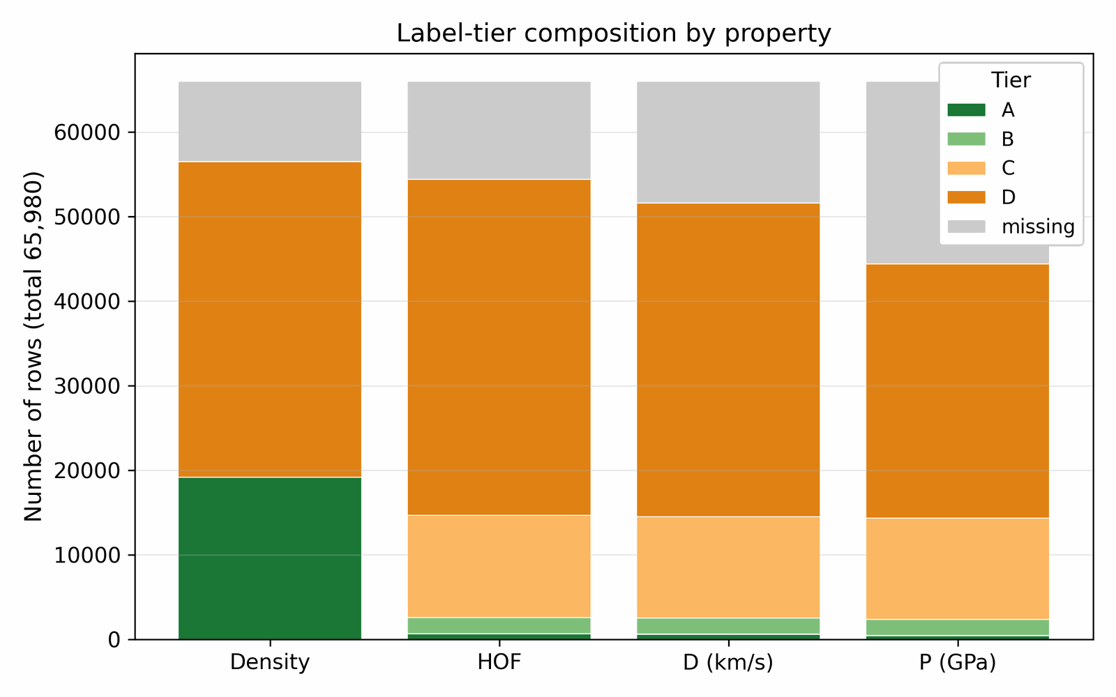
We assemble the training data by collecting molecules from several public sources that differ in both reliability and chemical scope. A small experimental core carries detonation properties measured in the laboratory; a larger DFT-quality slice carries energies and densities from first-principles simulation; a wider Kamlet–Jacobs-derived layer carries closed-form estimates from quoted density and heat of formation; and a model-derived majority carries surrogate predictions from a 3D-CNN ensemble trained on the union of the higher tiers. Some sources are restricted to energetic CHNO and CHNOClF chemistry (a labelled master of \(\sim 66\) k canonical SMILES (note: the labelled master includes CHNOClF molecules; the Stage-1 SMARTS gate at output removes all halogens, so all reported leads are CHNO-only) with at least one measured property and a motif-augmented expansion that systematically substitutes nitro / nitramine / azide / tetrazole groups onto labelled scaffolds); others draw from broader chemistry corpora (an unlabelled energetic SMILES dump of \(\sim 380\) k from the same chemical domain) that the diffusion model uses only to learn the unconditional prior. Every row is canonicalised to a single RDKit canonical SMILES, deduplicated across sources, and tagged with a trust tier; each property label is then used according to its reliability via the conditioning-mask recipe of §3.1. After cross-source deduplication and token-length filtering, the merged pretraining pool comprises \(\sim 694\) k unique molecules (pre-deduplication: 66k labelled + 380k unlabelled CHNO + 1.08M motif-augmented expansions = 1.53M; after canonical-SMILES deduplication across all three pools: 694k unique molecules; the motif-augmented pool contributes ~230k survivors after dedup with the base two pools), of which \(\sim 66\) k carry at least one property label. The complete source provenance (per-source row counts, citations, license terms, role in the four-tier hierarchy), the canonicalisation and tokenisation pipeline, and the high-tail oversampling ratios used during training are documented in Appendix A.1 / D. Joint property distributions and per-property histograms over the labelled corpus are shown in Figs 3 and 4; the label-tier composition (Fig 5) sits alongside the four-tier table in §3.1; atom-composition statistics over a 30k subsample are shown in Fig A.1.

3.1 Four-tier label hierarchy

Available property labels in the energetic-materials literature span four orders of reliability, from a small core of experimental measurements to a large majority of model-derived estimates. A naive concatenation would let the noisiest tier dominate the conditional gradient and degrade calibration in the high-property tail; discarding the noisier tiers would throw away most of the training signal. We resolve this by annotating each property label with a trust tier and gating the conditional gradient accordingly: only Tier-A and Tier-B rows participate in the conditional signal, while Tier-C and Tier-D rows train the unconditional prior via classifier-free-guidance dropout (§4.3). Each label per row carries one of the following tiers:

The denoiser conditional gradient fires only on Tier-A and Tier-B rows; Tier-C and Tier-D rows train the unconditional prior via classifier-free-guidance dropout (§4.3). This recipe lets the full corpus shape the marginal density of the generative model without letting noisy labels contaminate the conditional gradient. Each row carries a graded tier weight \(\omega\in[0,1]\), with default values \(w_A=1.0\), \(w_B=0.7\), \(w_C=0.3\), \(w_D=0.1\); later sections gate the conditional gradient and weight the per-row loss by these values.

3.2 Canonicalisation and tokenisation

Every SMILES string is canonicalised with RDKit [22a] (a fixed traversal order so that the same molecule yields the same string regardless of how the source database wrote it), converted to SELFIES (a robust tokenisation in which every legal token sequence decodes to a chemically valid molecule), and tokenised to the LIMO alphabet. Tokenisation, alphabet size, and the per-source preprocessing pipeline are in Appendix A.2. This step is purely data-side: no learned parameters are fit here; the output is a token-tensor representation of the corpus that the model of §4 will consume.

3.3 Training-time high-tail oversampling

The labelled detonation-velocity distribution is sharply peaked around 7–8 km/s, so during training Tier-A/B rows above the 90th percentile are oversampled by 5×–10×; this asymmetric high-tail oversampling raises the mean predicted velocity of the top leads by 0.4 km/s relative to a uniform-sampling control. The oversampling ablation is in Appendix D.4. The two denoiser variants of §4.3 differ in which property tail they apply this oversampling to (HOF tail vs ρ/D/P tail).

4. Methodology

4.1 Overview and pipeline map

DGLD is a four-stage pipeline (Figs 6–15): an encode-once LIMO VAE (Fig 7) feeds a conditional latent DDPM denoiser (Fig 9), whose sampling trajectory (Fig 13) is steered by a multi-task score model trained offline (Fig 11), and whose decoded candidates are filtered by a SMARTS+Pareto rerank funnel (Fig 14). The rest of §4 is organised one subsection per diagram panel; small panels are paired (§4.6 covers Fig 10 and §4.7 covers Fig 11), and the post-decode pipeline is split across three subsections (§4.9 Sampling covers Fig 13, §4.10 Filtering covers Fig 14, §4.11 Pool fusion covers Fig 15). §4.12 documents how every numeric constant in §4.2–§4.11 was selected. LIMO encoding is run once and cached, so all training and sampling happens in latent space; the decoder is invoked only at the end to read candidates back as SMILES. The conditional gradient is restricted to Tier-A and Tier-B rows; Tier-C and Tier-D rows drive the unconditional CFG branch only (§3.1, §4.3).

4.2 LIMO fine-tuning and one-time latent caching

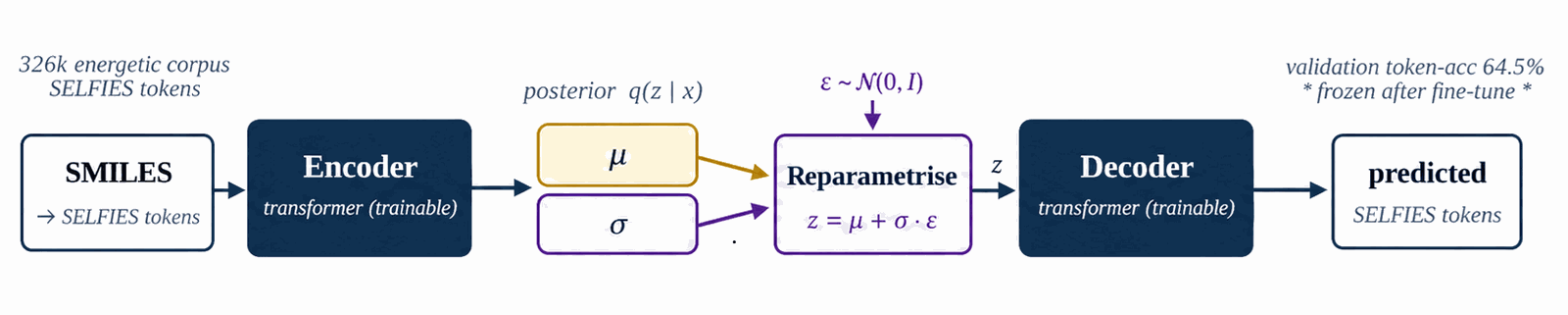
LIMO is the molecular-text VAE that supplies the cached latent μ used everywhere downstream. We fine-tune the pretrained checkpoint on the 326k energetic corpus to specialise the encoder, then freeze it for the rest of the pipeline. Sampling during fine-tuning is uniform; high-tail oversampling lives at the §4.4 denoiser-training stage and is not applied here.

We start from the pretrained LIMO checkpoint distributed with [1]. The encoder maps a (B, 72) SELFIES-token tensor through a 64-dim embedding and a four-layer MLP (Linear(72·64→2000)–ReLU–Linear(2000→1000)–BN–ReLU–Linear(1000→1000)–BN–ReLU–Linear(1000→2·1024)) to a (B, 1024) Gaussian latent (the final 2·1024 head packs μ and log σ²); the decoder mirrors this with Linear(1024→1000)–BN–ReLU–Linear(1000→1000)–BN–ReLU–Linear(1000→2000)–ReLU–Linear(2000→72·108) and produces a (B, 72, 108) log-probability tensor in parallel (no autoregression). Layer-by-layer widths and parameter counts are in Table B.1a. We fine-tune all parameters for \(\sim\)8.5k steps on the 326 k energetic-biased SMILES corpus with the standard ELBO, $$\mathcal{L}(x) \;=\; -\mathbb{E}_{q(z|x)}[\log p(x|z)] \;+\; \beta \cdot \mathrm{KL}(q(z|x) \,\|\, \mathcal{N}(0,I)),$$ with \(\beta=0.01\) and free-bits clipping disabled. After fine-tuning, validation token-accuracy is 64.5 %. The LIMO decoder is non-autoregressive (parallel decode); SELFIES syntax guarantees token-level validity, so molecule-level (full-sequence) validity is 100% by construction. Reconstruction accuracy (fraction of latent round-trips that reproduce the input SMILES exactly) is 31.4% on the energetic validation set, consistent with the expected LIMO performance in this domain. The latent posterior is concentrated: \(\|\mu\|\approx 8\) on average, well below the \(\sqrt{1024}\approx 32\) expected of \(\mathcal{N}(0,I)\).

After fine-tuning the encoder is frozen and every row of the data corpus (§3) is passed through it once to produce a deterministic latent mean \(\mu \in \mathbb{R}^{1024}\). The cached tensor stores, per row, the latent \(\mu\), a property matrix (the four conditioning targets \(\rho\), HOF, \(D\), \(P\)), a tier matrix, a per-row trust mask, and per-property normalisation statistics. The encoder posterior variance is discarded by design; \(\mu\) is treated as a deterministic anchor in latent space, and no SMILES is ever re-encoded at sample time. The denoiser of §4.3 and the score model of §4.7 read from this cached tensor only.

4.3 Conditioning mask construction

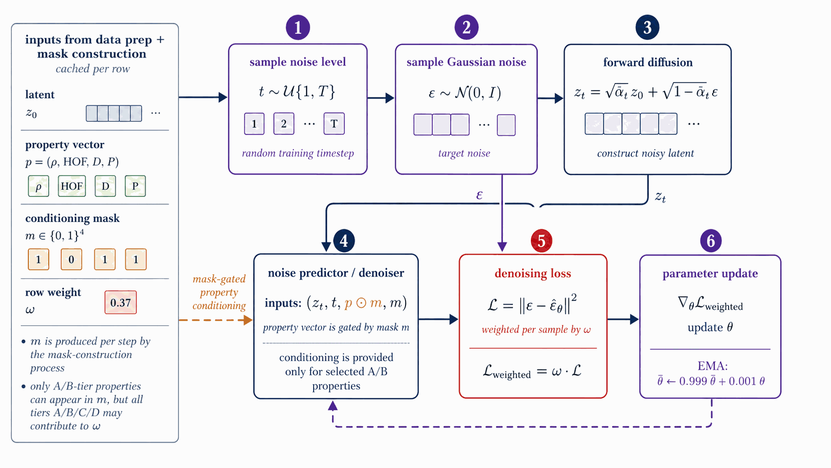
Each gradient step samples a fresh per-row mask m∈{0,1}⁴ that decides which of the four conditional properties are exposed to the denoiser at that step. The mask is the mechanism by which tier-eligibility (which labels a row carries) interacts with classifier-free dropout (the unconditional branch trained alongside the conditional).

The per-step training mask \(m\in\{0,1\}^4\) controls which conditioning properties enter FiLM at each step; the construction is a 5-stage stochastic pipeline over the per-row eligibility \(e\) and tier weight \(w_{\text{tier}}\) of §3.1 (distinct from the CFG scale \(w\) of §4.2).

Figure 8 walks the per-step mask construction. From cached eligibility \(e\in\{0,1\}^4\) (renamed from \(c\) to avoid collision with the conditioning vector) and the tier weight \(w_{\text{tier}}\) of §3.1, five stochastic stages produce \(m\): the subset-size box samples \(k\) from a Categorical with probabilities \(\{0{:}.10,\,1{:}.25,\,2{:}.30,\,3{:}.25,\,4{:}.10\}\); the weighted pick box samples \(k\) properties from \(e\) using \(w_{\text{tier}}\)-weighted multinomial draws to form a tentative one-hot; property dropout at rate 0.30 then independently zeros each entry of the tentative mask; CFG dropout at rate 0.10 zeros the entire mask to feed the unconditional branch.

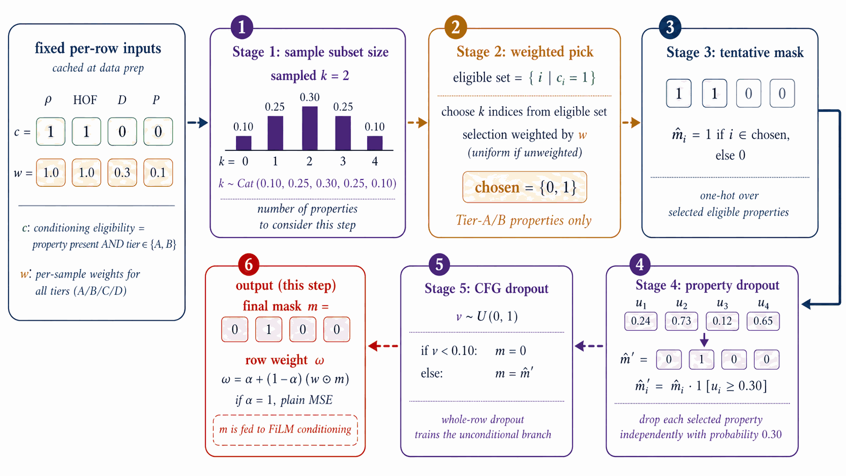
The output \(m\) and the row weight \(\omega_{\text{row}} = \alpha + (1{-}\alpha)\cdot\mathrm{mean}(w_{\text{tier}} \odot m)\) are emitted to the denoiser-training step of §4.4, where \(w_{\text{tier}}\) is the per-property tier-weight vector and \(\alpha \in [0,1]\) is the trust-vs-uniform interpolant (default \(\alpha=1.0\), reducing to plain MSE; \(\alpha < 1.0\) up-weights more-trusted rows). The mask \(m\) gates only the FiLM property input; it does not appear in the loss.

4.4 Denoiser training

The denoiser learns the noise-predicting reverse process of a 1000-step variance-preserving DDPM in latent space, conditioned via FiLM on the §4.3 mask + property vector. Classifier-free guidance dropout at training time enables the runtime trade-off between unconditional and target-property sampling controlled by the CFG scale w.

The denoiser \(\epsilon_{\theta}(z_t, t, c, m)\) is a 44.6 M-parameter FiLM-modulated ResNet over \(z_t \in \mathbb{R}^{1024}\) with 8 residual blocks of inner width 2048 (per-block: LayerNorm, Linear(1024 to 2048), FiLM(\(\gamma,\beta\) from cond), SiLU, Linear(2048 to 1024) with a residual add), a sinusoidal time embedding (\(d_t=256\)), and a sinusoidal property-value embedding (\(d_c=64\)) gated by the per-step mask \(m\in\{0,1\}^4\) of §4.3 (full hyperparameters in Table B.1b).

Figure 9 walks denoiser training. Per step: sample \(t \sim \mathcal{U}\{1{:}T\}\) and \(\varepsilon \sim \mathcal{N}(0,I)\); form \(z_t = \sqrt{\bar\alpha_t}\,z_0 + \sqrt{1-\bar\alpha_t}\,\varepsilon\) on the cosine \(T=1000\) DDPM schedule of Nichol & Dhariwal [dhariwal2021]; FiLM injects \((t,\,p\odot m)\); the network predicts \(\hat\varepsilon\); the loss is the per-sample MSE \(\Vert\varepsilon - \hat\varepsilon\Vert^2\) weighted by the row weight \(\omega_{\text{row}}\) of §4.3. Optimiser AdamW, peak LR \(10^{-4}\), cosine decay, batch 128, 20 epochs, EMA decay 0.999.

At sample time we use the standard guided estimate $$\hat\epsilon_{\theta}(z_t, c) \;=\; \epsilon_{\theta}(z_t, t, \emptyset) \;+\; w\,\big(\epsilon_{\theta}(z_t, t, c) - \epsilon_{\theta}(z_t, t, \emptyset)\big);$$ the production scale \(w = 7\) is selected per §4.12 (Figure 16).

4.5 Two complementary denoisers

The headline pipeline targets \(\rho\), \(D\), \(P\), and HOF simultaneously. Their labelled-corpus marginals have sharply different population statistics: the high-HOF tail and the high-\(\rho DP\) tail barely overlap in latent space. A single denoiser must compromise between these tails. Either tail can be trained to saturate, but not both at once with one loss-weighting schedule. We therefore train two complementary denoisers, each tilted toward one tail via training-time oversampling, so that each saturates its own tail.

DGLD-H tilts toward the HOF tail (asymmetric high-tail oversampling on Tier-A/B, factor 5×, focused on heat of formation). DGLD-P tilts toward the \(\rho DP\) tail (Tier-A/B-only conditioning, +5× high-tail oversampling on the top decile of the joint \(\rho/D/P\) distribution, weighted_mask=true, property-dropout 0.30). Both are 44.6 M-parameter FiLM-ResNets with the §4.4 architecture; only the training-data tilt differs. Hyperparameters of both checkpoints are listed in Table B.1b.

Empirically DGLD-H supplies high-HOF leads and DGLD-P supplies high-\(\rho/P\) leads. Combination happens post-decode in §4.11 (Figure 15): we union the lanes' SMILES pools and run them once through the rerank funnel. We do not average outputs or interpolate weights, so this is not a classical ensemble in that sense.

4.6 Labeling for guidance-head training

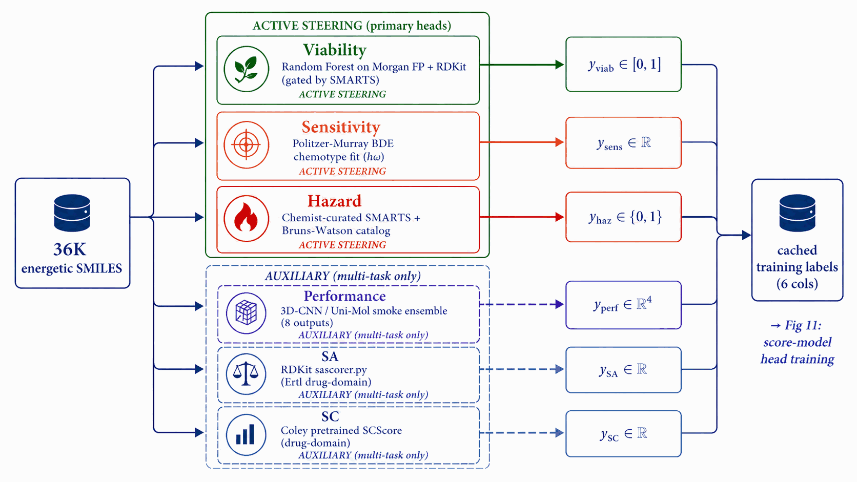
Each score-model head needs per-row training labels. We run six independent label-source pipelines once over the corpus, before any score-model training begins. Three feed active steering signals (Viability, Sensitivity, Hazard) with energetic-domain or rule-based labels; three feed auxiliary multi-task heads (Performance, SA, SC) with smoke-ensemble or drug-domain labels.

Each head plays a distinct role. Viability is the gatekeeper gradient that steers away from non-energetic regions; Sensitivity and Hazard are the safety axes the user cares about. These three are the active steering signals invoked at sample time. Performance, SA, and SC are auxiliary multi-task heads: trained on the shared trunk for regularisation but not invoked in the steering bus. Stage 2 of the Figure 14 reranker uses the 3D-CNN smoke ensemble (§4.10) for property scoring, not the latent Performance head.

Figure 10 walks the base label pipelines. A Random Forest on Morgan FP + RDKit descriptors yields \(y_{\text{viab}}\); a Politzer–Murray BDE chemotype-class fit on Huang & Massa [58a] \(h_{50}\) data yields \(y_{\text{sens}}\) (y_sens ∈ [0,1] with 1 = high sensitivity / dangerous; guidance descends this signal to reduce predicted sensitivity); the chemist-curated SMARTS catalog plus the Bruns–Watson demerit list yields \(y_{\text{haz}}\); and a 3D-CNN/Uni-Mol smoke ensemble yields \(y_{\text{perf}} \in \mathbb{R}^4\) over \((\rho, D, P, \mathrm{HOF})\). The cached LIMO \(\mu\) is held separately for the noised-latent training of the score model. Random Forest probability is portable, smooth, and decoupled; see Appendix B.1.

4.7 Score-model training

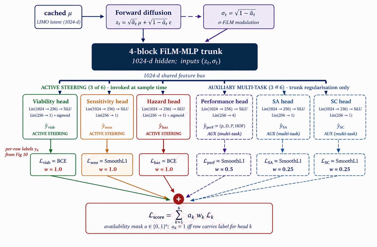
All six heads are trained jointly on a shared 4-block FiLM-MLP trunk under multi-task supervision. The trunk is regularised by all six losses; at sample time, only the three active steering signals are actually invoked. Auxiliary multi-task heads (Performance, SA, SC) earn their trunk-improving role during training but stay quiet during sampling.

The score-model trunk and six heads are trained on noised LIMO latents using the labels of §4.6 under multi-task supervision: three of the six (Viability, Sensitivity, Hazard) contribute steering signals at sample time, three (Performance, SA, SC) are auxiliary multi-task signals trained for trunk regularisation only.

Figure 11 walks score-model training. A shared 4-block FiLM-MLP trunk (1024-d hidden) consumes \((z_t, \sigma_t)\), where \(\sigma_t = \sqrt{1-\bar\alpha_t}\) is embedded into a 128-d sinusoidal token. Six heads branch off the trunk: Viability and Hazard are sigmoid heads trained with binary cross-entropy; Sensitivity, SA, and SC are smooth-L1 regressors; Performance is a 4-vector smooth-L1 regressor on \((\rho, D, P, \mathrm{HOF})\). Crucially, training data are noised latents at uniform \(t\), not clean \(\mu\), so the gradient is queried at every \(\sigma_t\) along the sampling trajectory. The total loss is the availability-mask-gated sum $$\mathcal{L}_{\text{score}} = \sum_k a_k \cdot w_k \cdot \mathcal{L}_k\bigl(\hat y_k(z_t, \sigma_t),\ y_k\bigr),$$ where \(a \in \{0,1\}^6\) is the per-head availability mask (distinct from the denoiser's per-property conditioning mask \(m \in \{0,1\}^4\) of Figs 8 and 9) and \(w_k\) are static head weights chosen so each \(\mathcal{L}_k\) sits at \(\mathcal{O}(1)\) at convergence (values in Table B.1b). Optimiser AdamW, peak LR \(2{\times}10^{-4}\), cosine decay, batch 1024, \(\sim\)40k steps, EMA decay 0.999.

The auxiliary multi-task heads (Performance, SA, SC) train on the shared trunk for regularisation only, not invoked in the production steering bus (Appendix B.4). Two checkpoint variants (production 6-head hazard-aware and its 5-head predecessor) are released on Zenodo (Appendix D.1).

4.8 Self-distillation refinement of the viability head

Round-0 viability labels combine SMARTS pass/fail with a Random Forest classifier trained on (energetic corpus, ZINC drug-like), a coarse two-class boundary. Self-distillation closes the gap between that boundary and the latent regions the diffusion sampler actually inhabits, by mining the model's own false-positive cheats and re-feeding them as labelled hard negatives.

The FROZEN banner of Figure 12 is read literally. Across all rounds the LIMO encoder, LIMO decoder, the §4.5 denoisers, the Random Forest, and the SMARTS rulebook do not retrain. The score-model trunk and heads are the only thing that updates between rounds. Within the score model, hard-negative latents are labelled \(y_{\text{viab}} = 0\) only; the other heads see those rows with \(a_k = 0\) (unlabelled).

The five-step protocol (sample → mine → encode → retrain → probe) is detailed in Appendix B.1. The hard-negative ticker on Figure 12 shows 0 \(\to\) 137 \(\to\) 918 cumulative negatives over rounds 0/1/2. (round-0 training uses 0 hard negatives; round-0 mining produces 137; round-1 training uses 137; round-1 mining cumulates to 918; round-2 / production training uses 918.)

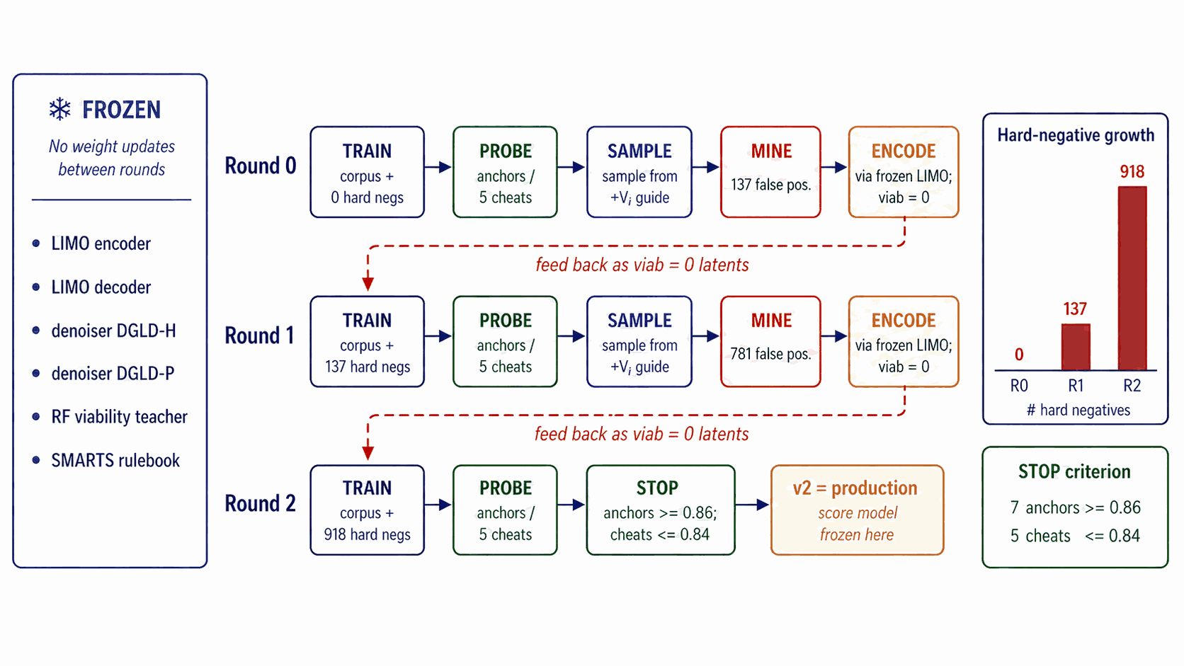
The stopping criterion is shown in the right-margin box of Figure 12: a held-out probe (7 anchors {RDX, HMX, TNT, FOX-7, PETN, TATB, NTO} and 5 cheats) must show every anchor at \(\ge\) 0.86 AND every cheat at \(\le\) 0.84. Empirically 3 rounds satisfy this; round 2 (corpus + 918 hard negatives) is the production checkpoint. Pseudocode in Appendix B.1.

4.9 Sampling

At sample time, three of the six trained heads (Viability, Sensitivity, Hazard) supply gradient steering signals at every DDIM step on top of classifier-free guidance. The denoiser remains the same checkpoint as §4.4; only the sampler changes.

Figure 13 walks sampling. A latent \(z_T \sim \mathcal{N}(0, I_{1024})\) is denoised over \(t = T \to 1\) in 40 DDIM steps. At each step, $$\hat\epsilon \;=\; \epsilon_\theta^{\text{cfg}}(z_t, t, c) \;-\; \sigma_t \sum_{h\in\{\text{viab},\text{sens},\text{hazard}\}} s_h\,\nabla_{z_t}\,\mathcal{L}_h\big(z_t,\sigma_t\big),$$ where \(\epsilon_\theta^{\text{cfg}}\) is the standard CFG noise estimate over the frozen denoiser of §4.5 (Figure 9). The per-head losses are \(-\log P_{\text{viab}}\) (ascend), \(\mathrm{sens}_z\) (descend), and \(-\log(1-P_{\text{hazard}})\) (descend hazard). Production scales are \(s_{\text{viab}}=1.0\), \(s_{\text{sens}}=0.3\), \(s_{\text{hazard}}=1.0\) (selection rationale in §4.12). The final \(z_0\) decodes through the frozen LIMO decoder to a SMILES pool consumed by Figure 15.

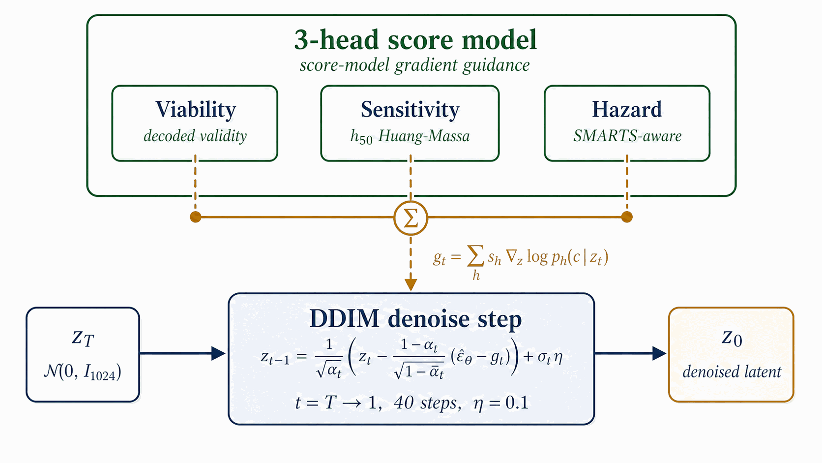
The classifier-guidance steering bus uses two configurable knobs: a noise-dependent annealing factor \(\alpha(\sigma_t) = \max(0,\,1 - \sigma_t/\sigma_{\max})\) that scales the bus down at high noise levels (where the score-model heads have not yet seen enough latent structure to be reliable), and a per-row gradient-norm clamp at magnitude \(C_g\) (gradient clamp) that prevents a single row from dominating the batch. The image-domain classifier-guidance recipe of Dhariwal & Nichol [15a] uses \(\sigma_{\max} = \sigma_T\) (full ramp on) and \(C_g = 5.0\); this works well at 1000 sampling steps, where each step covers a small \(\sigma\)-jump and the natural per-row gradient magnitudes sit well below 5. In the 40-step latent regime the same recipe zeroes the bus at the top of the trajectory (the first \(\sim\)10 steps live near \(\sigma_t \approx \sigma_T\)) and saturates the clamp at the bottom (natural gradient magnitudes at low \(\sigma\) are 8–30, well above 5), so the per-head scales \(s_h\) have negligible effect on the produced chemistry. Production disables the anneal by setting \(\alpha \equiv 1\) directly (equivalent to the \(\sigma_{\max} \to \infty\) limit of the schedule above; we configure this via a guard clause on \(\sigma_{\max}=0\) in code, treating it as the no-anneal sentinel) and loosens the clamp (\(C_g = 50\)). The four-test diagnostic that mapped per-step gradient norms across both configurations is in Appendix D.5. The CFG scale \(w\) is selected from the §4.12 sweep (Figure 16, \(w \in \{5, 7, 9\}\) at pool=8k); per-property quantile-error breakdown is in Appendix D.8.

4.10 Filtering

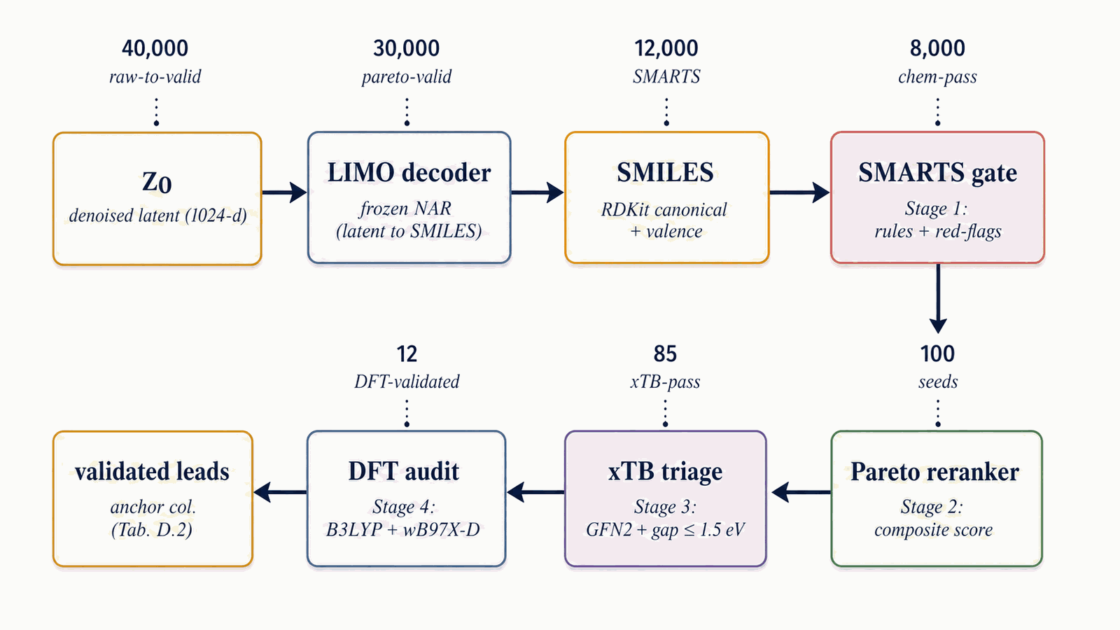
The decoded SMILES pool flows through a four-stage funnel that progressively raises the bar from cheap chemistry rules (SMARTS gate) to expensive first-principles audits (DFT). Stages 1+2 (ms cost per candidate) score every candidate; Stages 3+4 (CPU- and GPU-hours per candidate) run only on the top-K survivors.

Figure 14 walks the four-stage filtering funnel. Each pool is canonicalised, deduplicated, and stripped of charged species and over-large molecules. Stage 1: SMARTS gate (rules + redflags). A chemist-curated SMARTS [daylight-smarts] catalog removes radicals, sulphur, halogens, mixed valence states, and other red flags; survivors are scored by the 3D-CNN smoke ensemble. SA [19] \(\le\) 5.0 and SCScore [20] \(\le\) 3.5 caps are applied. Tanimoto similarity to the nearest training-set neighbour is required to lie within \([0.20, 0.55]\). Stage 2: Pareto reranker. The composite $$S(x) \;=\; 0.45\,S_{\text{perf}}^{\text{band}}(x) + 0.20\,S_{\text{viab}}(x) + 0.15\,S_{\text{novel}}(x) + 0.20\,(1-S_{\text{sens}}(x)) - 0.10\,S_{\text{alerts}}(x)$$ is computed, then a Pareto front over (\(-\)perf, \(-\)viab, sens, alerts) is used as the outer stratifier with the composite as within-stratum tiebreak. Default top-\(K=100\). The Stage-2 reranker draws property scores (\(\rho, D, P, \mathrm{HOF}\)) from the 3D-CNN smoke ensemble (via evaluate_candidates.py + rerank_v2.py), not from the latent Performance head; the latent Performance head trains as a multi-task auxiliary on the shared trunk for regularisation only and is not invoked at rerank time. Stage 3: xTB triage. GFN2-xTB optimisation, HOMO–LUMO gap \(\ge\) 1.5 eV (§5.3). Stage 4: DFT audit. B3LYP/6-31G(d) optimisation + \(\omega\)B97X-D3BJ/def2-TZVP single-point + 6-anchor calibration + Kamlet–Jacobs (§5.3). Illustrative survivors at the §5 production setting: pool=40k \(\to\) \(\sim\)1 800 chem-pass after Stage 1+2 (4.6 % keep-rate per §F.2) \(\to\) top-100 by composite re-rank \(\to\) 12 DFT-validated leads.

The Pareto-front procedure in Stage 2 is the four-step sweep:

1. Score each candidate with the composite \(S(x)\) defined above (perf-band, viability, novelty, sensitivity, alerts).
2. Mark each candidate as on-front or dominated, against the four-objective comparison (\(-\)perf, \(-\)viability, sensitivity, alerts) using a standard pairwise non-dominance sweep.
3. Sort with a two-key order: Pareto-front candidates first, then non-front; within each stratum by composite descending.
4. Return the top-\(K\) (default \(K = 100\)).

4.11 Pool fusion across sampling runs

A single sampling lane fixes one (denoiser, conditions, guidance) tuple. Pool fusion runs multiple lanes in parallel and unions their decoded SMILES outputs, exploiting the lanes' independent failure modes for diversity. The §4.10 reranker is what tie-breaks across the fused pool.

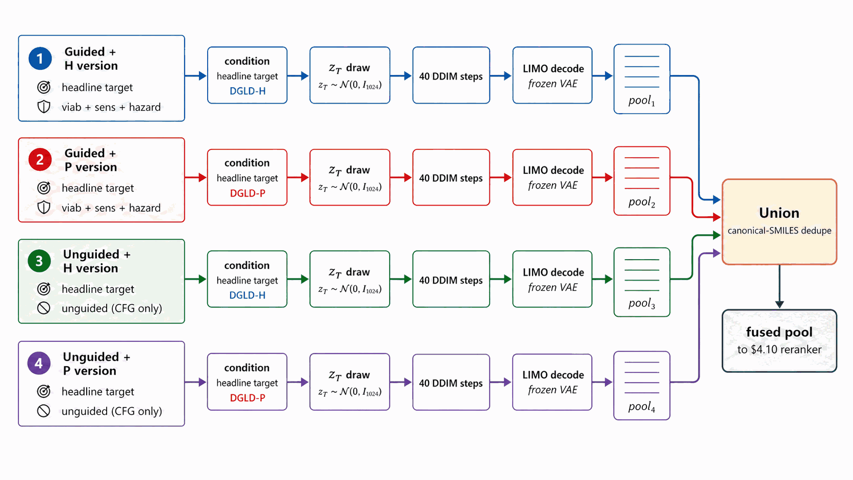
Figure 15 walks pool fusion. A single sampling lane = one (denoiser, conditions, guidance) tuple, run end-to-end (\(z_T\) draw \(\to\) 40 DDIM with that lane's config \(\to\) LIMO decode \(\to\) SMILES pool). The production methodology recipe is two lanes, one per denoiser (DGLD-H and DGLD-P), both at the headline target conditions, both at viab+sens+hazard guidance, both at CFG \(w=7\), pool \(\ge\) 40k each. Fusion is post-decode: the lanes' pools are unioned, canonical-SMILES deduplicated, and fed into the Stage-1 reranker. The three orthogonal diversity axes are conditions, denoisers, and guidance; each breaks a different correlated failure mode. The §F.4 four-pool merge (which adds two unguided ablation lanes) is a presentation choice for the merged top-100 result, not the production methodology recipe.

4.12 Training and hyperparameter selection

Every numeric constant in §4.2-§4.11 is selected by one of four mechanisms: empirically swept, stop-criterion-driven, inherited from prior work, or chemist-set. This section walks each bucket and flags what was empirically verified versus what was a defensible default.

Every numeric constant introduced in §4.2–§4.11 falls into one of four buckets, distinguished by how the value was set: empirical sweeps, stop-criterion-driven counts, values inherited from prior work, and chemist-set thresholds. The remainder of this section walks each bucket in turn, then closes with the limitations of the selection procedure.

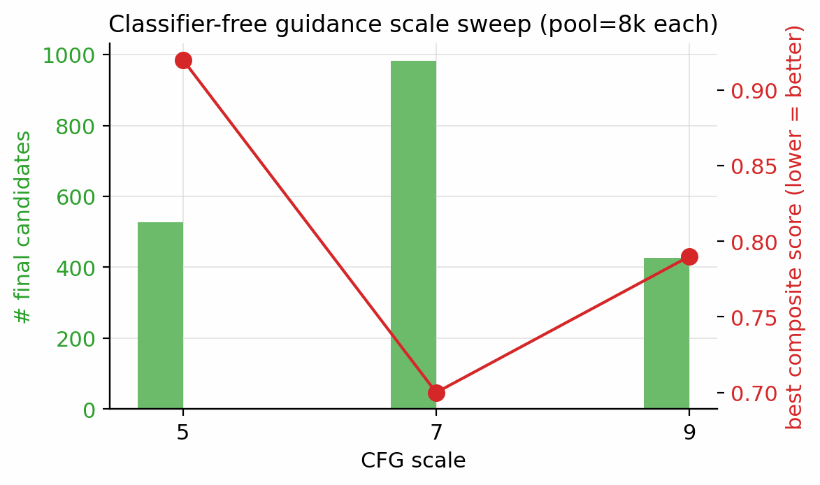
The first bucket is empirically swept. Two knobs were swept directly under the post-filter survival metric: the classifier-free-guidance scale \(w\) (Figure 16) and the candidate pool size (Figure 17). The CFG scale was tested at three points, \(w \in \{5, 7, 9\}\) at pool=8k, ranked by post-filter yield; \(w=7\) is the empirical sweet spot, with more candidates surviving than at \(w=5\) and the tight-mode collapse at \(w=9\) avoided. The pool-size sweep ranged from 1.5k to 40k, with both the best composite and the post-filter survival count still climbing at 40k; production uses pool \(\ge\) 40k per lane. The per-head guidance scales \(s_h\) were also empirically chosen via the §F.4 multi-axis matrix (full grid in Appendix D.6), and the score-head loss weights \(w_k\) were hand-set so each \(\mathcal{L}_k\) sits at \(\mathcal{O}(1)\) at convergence (ablation in Appendix B.3).

The second bucket is stop-criterion-driven. The self-distillation round count was set by the held-out probe described in §4.8, which requires every anchor at \(\ge\) 0.86 and every cheat at \(\le\) 0.84; the production budget-918 checkpoint is round 2 of self-distillation (round 0 = score-model trained on corpus only with Random-Forest-derived viability labels and 0 hard negatives, round 1 = corpus + 137 mined hard negatives, round 2 = corpus + 918 cumulative hard negatives + aromatic-heterocycle boost), the first to satisfy both conditions. The hard-negative count (918) is the cumulative round-2 mining yield, not a tuned target.

The third bucket is inherited from prior work or community convention and is not retuned in this paper. The KL weight \(\beta = 0.01\) is the LIMO original; the DDPM uses the cosine \(T = 1000\) schedule of Ho et al. [18]; the per-property dropout rate of 0.30 follows FiLM convention; the CFG dropout rate of 0.10 follows Ho and Salimans 2022; AdamW with peak LR \(10^{-4}\) on a cosine schedule plus EMA decay 0.999 is the standard diffusion-training recipe.

The fourth bucket is chemist-set thresholds, fixed by domain conventions rather than by sweep. The xTB HOMO–LUMO cut is \(\ge\) 1.5 eV; the DFT calibration set is the 6-anchor panel (RDX, TATB, HMX, PETN, FOX-7, NTO); the Tanimoto novelty window is \([0.20, 0.55]\) (operational novelty criterion for this pipeline; absolute scaffold novelty in the HEDM literature requires additional expert review); molecular-weight floor is 130 Da and the oxygen-balance cap is \(+25\,\%\).

The selection procedure has clear limitations. No Bayesian optimisation, no global grid search, no joint sweep over (\(w\), \(s_h\), pool size), and no per-target retuning are performed; all ablations reported in §5 and Appendix D are 1D. §5.6 hosts only the use of these settings (baseline comparisons, top-1 metrics) and Appendix D gives the full per-axis grids; the selection process lives here. The full compute footprint is summarised in Appendix D.2.

5. Experiments

5.1 Roadmap and headline targets

§5 is structured results-first: §5.2 reports the gated Pareto reranker top leads (Stages 1+2 of the validation chain); §5.3 reports physics validation (xTB triage and DFT confirmation, Stages 3+4); §5.4 combines novelty, retrosynthesis, and the E-set scaffold-diversity audit; §5.5 contrasts DGLD against no-diffusion baselines; §5.6 is the ablation summary. The four headline targets are \(\rho \ge 1.85\) g/cm³, \(D \ge 9.0\) km/s, \(P \ge 35\) GPa and Tanimoto novelty \(\le 0.55\) against every training row, validated through the four-stage chain SMARTS \(\to\) Pareto \(\to\) xTB \(\to\) DFT documented in §4.10 (Fig 14). Hyperparameters and the production configuration (CFG=7, pool \(\ge\) 40k per denoiser, alpha-anneal disabled) are documented in §4.12 and Appendix B.5 (Table B.5) and are not re-derived here.

5.2 Top leads from the gated Pareto reranker (Stages 1+2)

Applying the §4.10 gated multi-objective reranker (hard filters, banded performance score, viability, novelty, sensitivity, alerts) to the pool=40 000 candidate set: of the top-400 single-objective candidates, 45 are rejected by the hard filters (poly-nitro-on-C2, MW < 130, OB > +25 %); the 355 survivors define a Pareto front of 34 candidates (Fig 20). The top-five Pareto leads are shown in Figure 19. 89/100 of the merged top-100 originate from the smallest unguided pool reranked by the Pareto scaffold composite (the rank-1 trinitro-isoxazole itself comes from a guided run); guidance acts as a high-precision lever on the top of the funnel, not as the source of bulk Pareto coverage (source-pool breakdown in Appendix D.10).

The top-five leads (Figure 19, L1–L5) have viability 0.83–1.00, MW between 147 and 233 Da, and oxygen balance within ±15 %. Lead L1 is the aromatic trinitro-1,2-isoxazole, predicted at \(\rho=2.00\) g/cm³, \(D=9.56\) km/s, \(P=40.5\) GPa, comparable to HMX. The Pareto front contains 34 candidates with composite \(\ge\) 0.50 and viability \(\ge\) 0.83 (Fig 20). Naive single-objective ranking (without the gating layer) puts a polynitro-on-C2 model-cheat at the top; the gates correctly reject it (full SMARTS-trace and rejected-candidate property tabulation in Appendix D.7).

5.3 Physics validation and DFT confirmation (Stages 3+4)

Stage 3 (xTB triage). The merged top-100 from Stages 1+2 is the input to Stage 3 GFN2-xTB triage at the 1.5 eV HOMO–LUMO gap gate: 85/100 survive, and 6/8 of the smaller production gated top-8 also survive. The xTB triage agrees with the §6 chemistry-expert critique: open-chain and strained spiro candidates fall out as low-gap, while the aromatic isoxazole and small saturated heterocycles survive cleanly. The full xTB recipe (RDKit ETKDGv3 + MMFF94 + xTB --opt tight) is in Appendix C.12. Pool-size dependence: repeating the xTB triage on the gated top-15 of an unguided pool=80 000 run, 13/15 survive the same gate, indicating that classifier guidance can drive the sampler into modes that score high on learned proxies but fail at frontier-orbital electronic stability; a larger unguided pool with the same gating produces a more physically-credible final set.

Stage 4 (DFT audit). First-principles DFT audit at B3LYP/6-31G(d) optimisation + \(\omega\)B97X-D3BJ/def2-TZVP single-point on the 12 chem-pass leads alongside two anchors (RDX, TATB) using GPU4PySCF (density from Bondi van-der-Waals integration with packing 0.69). All twelve chem-pass leads + two anchors are real local minima (no imaginary frequencies; min real modes 9–52 cm⁻¹); three SMARTS-rejected reference scaffolds (R2, R3, R14) optimised under the same protocol are in Appendix C.5. The 73 candidates that pass Stage 3 but not Stage 4 are accounted for in Appendix C.5 (45 rejected by Stage 2 hard filters; 28 fail K-J/imaginary-frequency/composition gates).

6-anchor calibration. A linear 6-anchor (RDX, TATB, HMX, PETN, FOX-7, NTO) calibration gives \(\rho_{\text{cal}} = 1.392\,\rho_{\text{DFT}} - 0.415\) and HOF\(_{\text{cal}} = \)HOF\(_{\text{DFT}} - 206.7\) kJ/mol, with leave-one-out RMS \(\pm 0.078\) g/cm³ on \(\rho\) and \(\pm 64.6\) kJ/mol on HOF (full intercept derivation in Appendix C.1–C.3). Calibrated densities span \(\rho_{\text{cal}} \in [1.84, 2.09]\) g/cm³; L1 raw DFT \(\rho_{\text{DFT}}=1.80\) calibrates to \(\rho_{\text{cal}}=2.09\) g/cm³ (the highest of the set), and its raw HOF\(_{\text{DFT}}=+229.5\) kJ/mol calibrates to \(+22.9\) kJ/mol.

Kamlet–Jacobs recompute and headline corroboration. Two K-J applications appear: (i) per-lead calibrated branch (Table 3): K-J on DFT-calibrated \((\rho_{\text{cal}},\,\text{HOF}_{\text{cal}})\) for ranking; (ii) population residual branch (Table C.4): K-J on raw experimental \((\rho,\,\text{HOF})\) from 575 Tier-A labelled rows to quantify K-J under-prediction at high N-fraction. Calibrated K-J velocities span \(6.71\)–\(8.25\) km/s across the 12 chem-pass leads. L1 calibrated K-J \(D = 8.25\) km/s; the 1.31 km/s residual to the 3D-CNN surrogate (9.56 km/s) is larger than the K-J anchor residuals in L1's own composition regime (L1: \(f_N \approx 0.29\), OB \(\approx +8\,\%\), placing it in PETN's K-J-reliable regime, not the high-N RDX/HMX/FOX-7 under-prediction band). Note that L1's OB sits at the upper boundary of the standard oxygen-deficient regime (\(d = 2a + b/2 = 6\) vs L1's \(d = 7\)); we apply Kamlet–Jacobs in its unified product-distribution form (the standard treatment for mildly oxygen-rich CHNO; see Kamlet–Jacobs 1968 §III). The 1.31 km/s gap is therefore plausibly 3D-CNN surrogate over-prediction in the sparsely-represented polynitroisoxazole region rather than K-J failure. The DFT-K-J recompute places L1 in the HMX-class regime by relative ranking against anchors; absolute \(D\) values require a thermochemical-equilibrium covolume solver (§6). Full K-J residual decomposition (PETN/NTO chemistry; \(r(f_N,\text{residual})=+0.43\), \(p = 4\times 10^{-27}\) on 575 Tier-A rows) is in Appendix C.6–C.7. An independent Cantera ideal-gas CJ recompute ranks L1, L4, L5 as RDX-class; absolute \(D\) values require BKW/JCZ3 covolume corrections (§6), full discussion in Appendix C.13.

Cross-check on SMARTS-rejected candidates. The same DFT pipeline applied to three of the 23 SMARTS-rejected candidates (rank-2 N-nitroimine, rank-3 polyazene, rank-14 azo-amino-nitrate) finds them to be real geometric minima at B3LYP/6-31G* (min real frequencies 33–47 cm⁻¹). The chemist rejection is motif-level (shock-sensitivity, friction-trigger risks beyond gas-phase DFT), not geometric: the SMARTS and DFT layers are complementary, not redundant. The hazard-head post-hoc filtering recovers all 23 SMARTS rejects with perfect recall by construction and exposes 66 additional candidates on which the SMARTS catalog is silent (Appendix D.12).

Literature context for L1. The polynitroisoxazole family is established in the energetic-materials literature ([sabatini2018][tang2017]); the isomeric 3,4,5-trinitro-1H-pyrazole [herve2010] is the closest fully-substituted ring previously characterised. The 3,4,5-trinitro-1,2-isoxazole isomer DGLD proposes is absent from the 65 980-row labelled master (max-Tanimoto 0.27) and from PubChem; it is therefore a chemotype-class rediscovery with a positionally novel substitution pattern.

5.4 Novelty, synthesisability, and scaffold diversity

Three audits frame the merged top-100 against PubChem, public USPTO retrosynthesis templates, and a scaffold-distinct E-set extension. The headline is that DGLD generates a chemotype distribution (10 DFT leads / 8 Bemis–Murcko scaffolds / 6 families), not a single isoxazole hit.

Novelty audit

Of the merged top-100, 96/97 are absent from PubChem [23] (PUG REST on canonical SMILES; 3 transient REST errors excluded; the one rediscovery is 1-nitro-1H-tetrazol-1-amine at rank 56). Independently, 97/100 are absent from the 65 980-row labelled master; the three rediscoveries (dinitramide, 1,2-dinitrohydrazine, N,N′-dinitrocarbodiimide) confirm the model rediscovers established high-density CHNO motifs. Zero of the 100 candidates lie within Tanimoto 0.70 of any training row, and zero are exact matches in the 694 518-row augmented corpus (Table 4); the candidates are more distant from the augmented corpus than from the labelled master alone, despite the augmented corpus being >10× larger. The strengthened SMARTS catalog (N-nitroimines and open-chain polyazene/azo-nitro motifs) retains 77/100 of the merged top-100; the rank-1 trinitro-isoxazole survives (per-class breakdown in Appendix D.7).

Retrosynthesis audit

AiZynthFinder [68] with public USPTO expansion + filter policies and the ZINC in-stock catalog (200 MCTS iter, 300 s/target) was applied to L1, L4, L5 and then extended to the remaining nine chem-pass leads. L1 returns 9 productive routes; the top route is 4 steps with state score 0.50 (Table 5). L4, L5, and the nine extension leads return zero productive routes within budget; reproduced at 5× budget (1000 MCTS iter, 1800 s) on L4/L5. The L1 disconnection sequence (electrophilic ring-nitration; Boc protection; DPPA-mediated Curtius rearrangement on 4,5-dinitro-1,2-isoxazole-3-carboxylic acid), its hazard caveats (acyl-azide intermediate at primary-explosive class), and the ZINC catalog gap on energetic-domain intermediates are documented in Appendix D.14. The 1/12 hit rate quantifies a public-USPTO drug-domain template-database gap, not unsynthesisability of the candidates; an energetics-domain template extension is flagged as community follow-up in §6.

E-set scaffold-diversity audit (E1–E10)

To probe scaffold diversity beyond the single sampling stream of the L-set, we mined a 500-candidate extension pool from the four sampling runs of §5.2 under the same Stage 1 SMARTS gate but with a Tanimoto-NN cap of 0.55 against L1–L20. The 500 SMILES were pre-screened with GFN2-xTB on Modal CPU; 10 scaffold-distinct survivors were promoted to A100 DFT under the same protocol used for L1–L20 and post-corrected with the 6-anchor calibration. By Bemis–Murcko bookkeeping the 10 picks span 8 distinct scaffolds across 6 chemotype families: 1,2,3,5-oxatriazole (E1), NH-pyrrole nitroaromatic (E6), acyclic and small-ring nitramines (E2–E4), small-ring nitrate esters (E5, E7), geminal polynitro carbocycle (E8), bare 1H-tetrazole (E9), and nitro-imidazoline (E10); four families (oxatriazole, NH-pyrrole, acyclic nitramine, geminal polynitro carbocycle) are absent from the L-set entirely.

†E2 D and P are flagged: OB = +28.9 % exceeds the +25 % K-J reliability limit; these values are upper-bound estimates only (see §5.4 E2 audit). E9 K-J is undefined (OB < −200 %).

E1 oxatriazole as a co-headline finding. Under the same 6-anchor calibration applied to L1, E1 (4-nitro-1,2,3,5-oxatriazole) reaches \(\rho_{\text{cal}} = 2.04\) g/cm³, \(D_{\text{K-J,cal}} = 9.00\) km/s, \(P_{\text{K-J,cal}} = 38.6\) GPa, with a Politzer–Murray BDE-correlated h₅₀ of 82.7 cm; both E1's calibrated \(D\) and \(\rho\) are higher than L1's. The 1,2,3,5-oxatriazole ring system has known thermal/Lewis-acid ring-opening pathways (Sheremetev 2007; Katritzky 2010); a dedicated BDE and DSC/TGA stability screen is required before E1 is promoted to synthesis priority (Appendix C.5 caveat block). Two honest readings of E1's headline number are possible without an oxatriazole-class anchor: (i) E1 is genuinely stronger than L1, giving the paper two HMX-class leads from disjoint chemotype families; or (ii) the K-J residual is chemotype-dependent and E1 is upper-bounded until an oxatriazole-anchor recompute (a thermochemical-equilibrium CJ on calibrated inputs and an oxatriazole-class anchor extension are scoped as future work in §6).

Of the 10 E-set candidates, 4 of 9 with defined K-J clear \(D_{\text{K-J,cal}} \ge 7.0\) km/s (E1–E4); 8 of 9 have h_50BDE \(\ge\) 30 cm. E9 (bare 1H-tetrazole) is a deliberate filter-check: K-J is undefined at its oxygen balance and Stage 4 correctly leaves \(D\) and \(P\) unreported. E2's K-J \(D\) (9.22 km/s) is upper-bound only because its OB = +28.9 % exceeds the +25 % K-J reliability limit (Appendix D.13). The L-set sits at the upper edge of a credible distribution; L1 and E1 are two HMX-class picks from chemically distinct families.

5.5 Comparison with no-diffusion baselines

Four no-diffusion baselines were run through the same downstream pipeline on the same training corpus to isolate the contribution of the diffusion prior and guidance. The Gaussian-latent control and the matched-compute guided-vs-unguided headline are reported in §F.2 and §F.3 respectively. Results are in Table 8 and Figure 22.

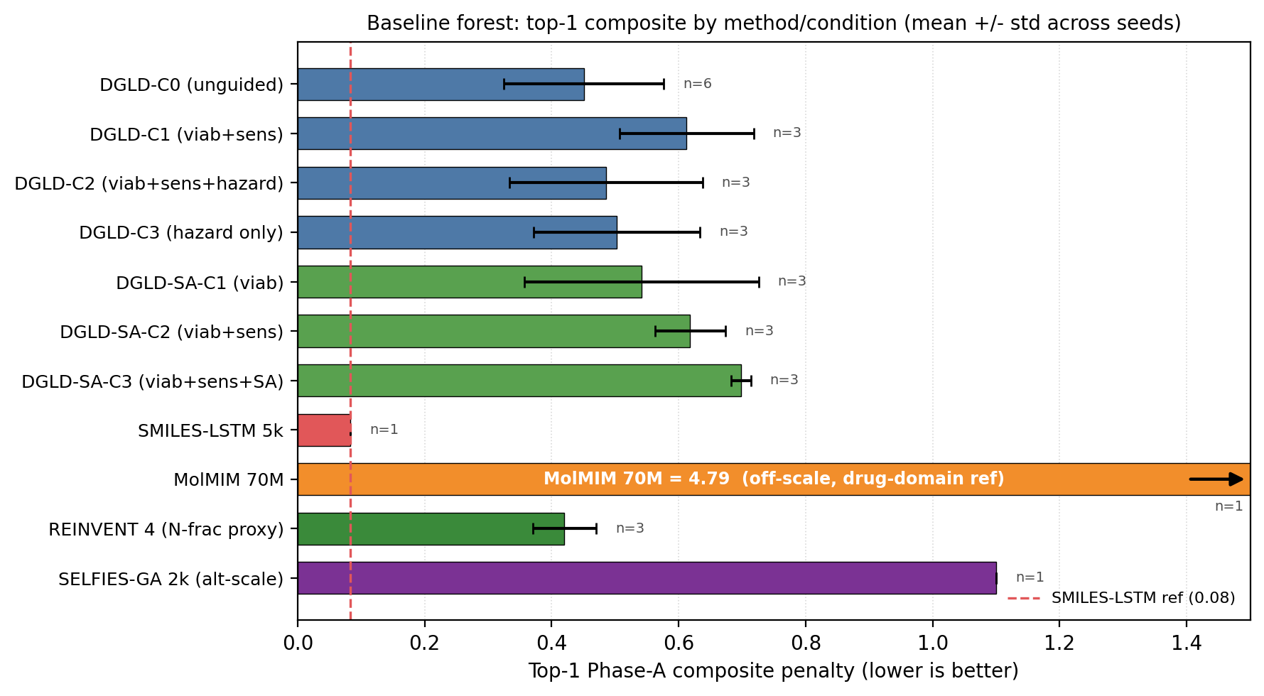
SELFIES-GA collapses under DFT audit. SELFIES-GA (2k-molecule pool, 30 generations) returns 75/100 top candidates as exact corpus rediscoveries (top-1 is a rediscovery); the best novel candidate at 2k is rank 5 (\(D=9.39\) km/s, max-Tanimoto 0.487); at 40k pool, the best novel outlier reaches \(D_{\text{surrogate}}=9.73\) km/s but collapses to \(D_{\text{DFT}}=6.28\) km/s under the same DFT audit chain applied to DGLD leads (3.5 km/s surrogate artefact; the 3D-CNN is not calibrated for nitro-oxadiazole/triazole fused scaffolds). SMILES-LSTM (2-layer, 6 M parameters, trained on the same 326 k SMILES corpus): top-1 is an exact labelled-master rediscovery (max-Tanimoto = 1.000); memorisation rate 18.3% ± 0.5% across 3 seeds, seed-stable. The best novel top-1 is a 5-atom aminotriazole fragment with no 3D-CNN score; the model reproduces training data, not new energetic leads. MolMIM 70 M (drug-domain pretrained): top-1 novel at Tanimoto 0.625 but at \(D=7.70\) km/s, far below HMX; uncalibrated for the energetic regime. REINVENT 4 (N-fraction RL reward, 3 seeds, 40k pool): generates genuinely novel high-N heterocycles with exact memorisation below 0.1%; seed-42 top-100 Uni-Mol-scored at top-1 \(D=9.02\) km/s, 0.37 km/s below DGLD Hz-C2. N-fraction RL is a useful novelty lever but does not optimise directly for the D/ρ/P targets DGLD conditions on. DGLD Hz-C2 is the only condition with consistent novel productive-quadrant coverage confirmed at DFT level. Appendix E lists the ten most-novel candidates from each baseline pool.

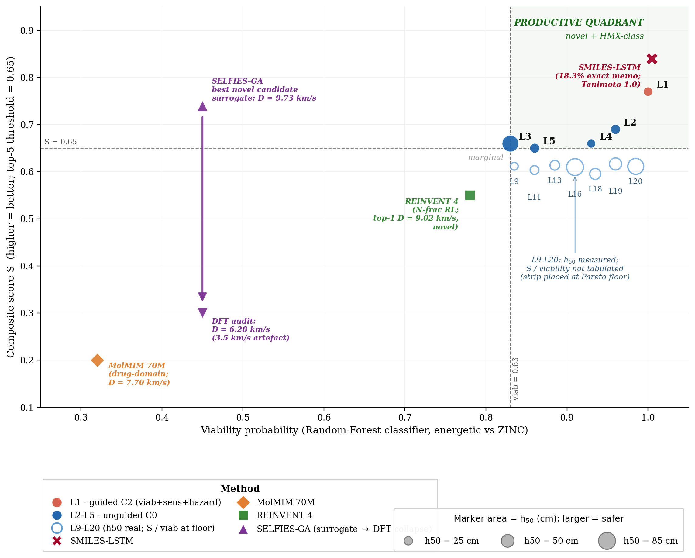
Note on Fig 23 score conventions. The composite score \(S\) on the \(y\)-axis is the higher-is-better Stage-1+2 reranker success score (range 0–1), not the lower-is-better Pareto-reranker penalty tabulated in Table 8, Fig 22, and Table F.4. Cross-figure ranking is consistent (DGLD Hz-C2 best on both) but absolute values are not comparable.

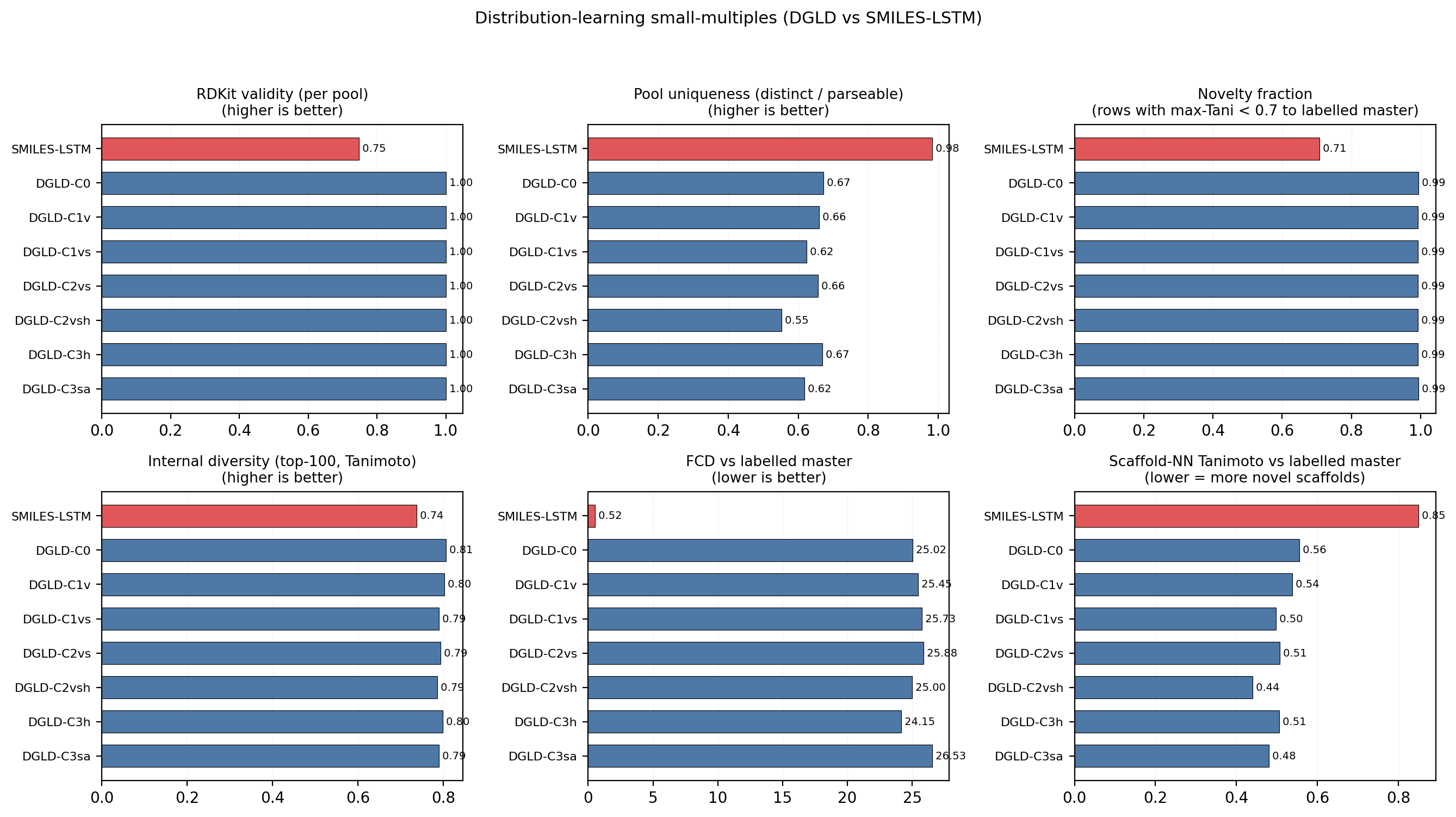
Distribution-learning metrics. SMILES-LSTM has FCD = 0.52 against a 5 000-row labelled master sample (distributionally indistinguishable because it reproduces labelled rows); DGLD has FCD = 24–26 across guidance conditions: the diffusion sampler performs a targeted search off the prior, not corpus mimicry, with anti-correlation between FCD and Pareto-reranker composite within DGLD confirming the design intent. Full small-multiples (validity, scaffold uniqueness 659–1262, IntDiv1 0.818–0.838) are in Appendix D.11.

5.6 Ablation summary

Seven ablations measure the contribution of each system component to the headline. Table 9 lists the headline result of each; full prose, sub-tables, and figures are in Appendix F. The forest plot of effect sizes (Figure 25) summarises the guidance-axis ablations visually.

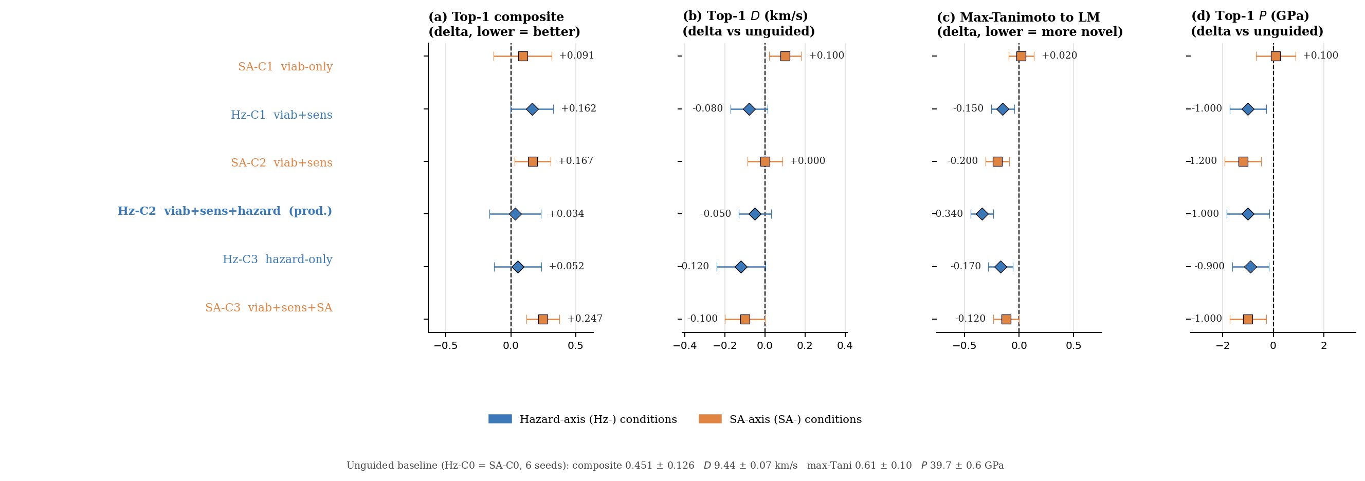
What each component contributes. The tier-gate is the single largest contributor: removing it collapses the sampler to high-N degenerate open chains (53.9 % keep-rate, no ring chemistry) rather than the ring-bearing high-density manifold the production model occupies. The diffusion prior contributes a +0.45 km/s \(D\)-lift over a compute-matched Gaussian-latent control, whose 48 % vs 4.6 % keep-rate reversal confirms that the diffusion prior's role is not chemical-plausibility filtering (a Gaussian decode through frozen LIMO does that easily) but distribution concentration on the high-\(D\) tail. Multi-head guidance trades scaffold diversity for novelty: hazard-axis C2 reaches max-Tanimoto 0.27 (the most novel condition) at the cost of scaffold count 5 vs 12. Pool fusion across 5 lanes lifts post-filter yield nearly five-fold (4 639 vs 966 candidates, +5\(\times\)) without lifting top-1, surfacing 24 Bemis–Murcko scaffolds vs 7.

Seed-variance context for the headline. Per-condition seed variance (3-seed s.d. on top-1 composite, range 0.106–0.184) is comparable to the across-condition mean differences, so the production C2 default is justified by the most-novel result rather than a sharp performance lift; the qualitative ablation conclusions are robust to seed across all six guidance axes (Table F.4, full multi-seed table). The 6-seed unguided baseline gives the tightest mean (top-1 composite 0.451 ± 0.126); the SA-axis SA-C3 (viab+sens+SA) is the worst at 0.698 ± 0.015.

What is ruled out. A drug-domain SA-gradient head (RDKit SAScorer, calibrated on Reaxys/pharma reaction corpora) worsens the composite by 13 % in our energetic-materials regime; production therefore uses \(s_{\text{SA}} = 0\). The SC head is retained as an architectural slot for backward compatibility but is not plumbed into the sample-time gradient sum. Both heads add \(\sim\)2 × 256k parameters of trunk-regularisation supervision during training (Appendix B.4 contains the full SA / SC drug-domain transfer-head story).

6. Limitations

Crystal packing is the dominant unquantified error source. All densities are estimated from gas-phase DFT geometry using Bondi van-der-Waals volumes with a fixed packing factor of 0.69. This factor varies from approximately 0.65 (loosely packing aromatics) to 0.72 (cubane-class compounds), with literature reports up to 0.78 for the densest CHNO crystals (§C.3); a ±5% packing-factor error alone propagates to ±0.10 g/cm³ in density, which at the K-J sensitivity of \(\partial D / \partial \rho \approx 2.9\) km/s per g/cm³ (Table 3) yields ±0.4 km/s in \(D\), roughly twice the 6-anchor calibration uncertainty of ±0.23 km/s. Note that this propagation applies to the uncalibrated Bondi-vdW estimate; the 6-anchor empirical calibration absorbs most of the systematic packing-factor error and brings the residual to ±0.078 g/cm³ (§C.4). Polymorph screening is absent; high-nitrogen heterocycles frequently exhibit multiple crystal forms with different densities and sensitivity profiles (cf. \(\varepsilon\)- vs other CL-20 polymorphs). Crystal structure prediction or experimental single-crystal X-ray diffraction is the critical missing step before any density-based performance claim can be considered quantitative. Crystal structure prediction is the natural follow-up validation; recent benchmarks of CSP on energetic molecular crystals (Crystal Growth & Design 2023, DOI:10.1021/acs.cgd.3c00706) demonstrate that polymorph screening is feasible at this candidate-list scale.

Independent cross-checks on L1 and E1. Two independent semi-empirical cross-checks confirm conservative bounds. A Bondi-vdW packing-factor bracket on L1 and E1 (Appendix C.9) yields \(\rho \in [1.69, 1.87]\) g/cm³ for L1 and \([1.65, 1.83]\) g/cm³ for E1, both below the 6-anchor-calibrated values (2.09 and 2.04); the 14% offset reproduces the calibration slope and confirms the pure Bondi-vdW estimator is conservative. A coordinate-preserving GFN2-xTB BDE scan (Appendix C.10) places the weakest-bond cleavage of L1 at 86 kcal/mol and E1 at 93 kcal/mol, both on C–NO₂ nitro-loss channels with no sub-80 kcal/mol channel that would predict primary-explosive sensitivity.

The 3D-CNN surrogate is well-calibrated on the labelled distribution but extrapolates onto the high-density tail with unquantified reliability; the top leads should be treated as candidates for DFT and experimental validation, not as final answers. SA and SCScore are heuristic synthesisability bounds. Absolute \(D\) values are reported under the closed-form Kamlet–Jacobs approximation; absolute-value-grade numbers require a thermochemical-equilibrium CJ code with a covolume EOS (EXPLO5, Cheetah-2, or the open-source Cantera-based Shock and Detonation Toolbox), which we do not run in this work. The six DFT anchor compounds contain no oxatriazole-class member; E1's \(D_{\text{K-J,cal}} = 9.00\) km/s is therefore an extrapolation outside the anchor chemical space. A 7th-anchor extension attempt with DNTF (Appendix C.11) failed and the 6-anchor calibration is retained; an oxatriazole-class anchor with experimental crystal density and detonation data remains scoped as future work before E1 reaches L1 confidence. L1's \(\rho_{\text{cal}} = 2.09\) g/cm³ also involves nitroisoxazole chemotype extrapolation: a packing factor of 0.65 (lower-end aromatic, vs 0.69 used) would give \(\rho \approx 1.97\), shifting \(D_{\text{K-J}}\) by roughly \(\pm 0.3\) km/s.

The 1.5–2 km/s Kamlet–Jacobs vs 3D-CNN residual reported in §5.3 is consistent with the typical disagreement between Kamlet–Jacobs and full Chapman–Jouguet thermochemical-equilibrium codes (EXPLO5, Suceská et al.; Cheetah-2, Fried–Howard) on high-N CHNO compounds: published benchmarks place this disagreement in the 0.3–1.5 km/s band for typical organic explosives and at the higher end (1–2 km/s) for compounds with N-fraction \(\gtrsim 0.4\), where the K-J fixed-product-distribution assumption breaks down. The population-level §5.3 evidence (Pearson \(r(f_N, \text{residual})=+0.43\), \(p<10^{-26}\)) is itself a regime-aware reproduction of the same effect on 575 Tier-A experimental rows. Definitive absolute-\(D\) numbers for the top lead therefore require either a thermochemical-equilibrium CJ recompute (EXPLO5, Cheetah-2, or the open-source Cantera SDT) on the calibrated DFT inputs, or experimental synthesis; the 3D-CNN \(D\) should be read as relative-ranking-grade, not absolute-value-grade.

Retrosynthetic accessibility under public USPTO templates is a known weakness for energetic-materials chemistry. AiZynthFinder finds a 4-step productive route only for L1 of the 12 DFT-confirmed leads. The 11 negative results reflect the drug-domain bias of the public template database (Reaxys-/USPTO-derived), not unsynthesisability of the candidates; energetic-domain templates (nitration, N₂O₅ nitrolysis, ring-cyclisation) would be required for an informative retro-screen.

The statistical scope of the headline numbers is bounded as follows. §F.4 reports a 4-condition × 3-seed head-to-head at pool=10k with a no-diffusion SMILES-LSTM baseline, and §F.3 reports the single-seed pool=40k head-to-head used for the merged top-100; tables elsewhere use a single sampling seed. 89/100 of the merged top-100 come from a single unguided pool reranked by the Pareto-reranker scaffold composite, so the headline novelty/stability numbers reflect this single sampling stream, with the multi-seed §F.4 matrix as the variance estimate. Each denoiser was originally one \(\sim\)6 hr training run; we have since retrained the v4b production architecture at two additional seeds and resampled the production C2 condition (Hz-C2 viab+sens+hazard, pool = 10k per seed). Across the resulting 3 denoiser seeds, top-1 \(D\) = 9.38 \(\pm\) 0.01 km/s (relative s.d. 0.1%), top-1 \(\rho\) = 1.92 \(\pm\) 0.01 g/cm³, top-1 \(P\) = 38.8 \(\pm\) 0.07 GPa. The denoiser-init seed variance is far smaller than the across-condition C0 \(\to\) C2 spread (\(\sim\)1% of mean), so the production C2 lift is not an artefact of a particular denoiser-init seed.

The diffusion model trains on the full 694k augmented corpus; the candidate-discovery objective is to extrapolate off the labelled distribution rather than recover held-out labels, so we do not report a held-out test split. The Tanimoto-stratified novelty against the 694k corpus (§5.4: median 0.32, 0/100 within Tanimoto 0.70) is the train-leakage proxy. The 3D-CNN surrogate → xTB triage → DFT minimum chain is not a substitute for first-principles equilibrium thermochemistry or experimental synthesis; we position the paper as a methodology and a candidate-list paper, not a synthesis paper. Finally, the cfg-dropout (0.10), property-dropout (0.30), high-tail oversample (10×), and the Tanimoto window (0.20, 0.55) are fixed configuration; no full hyperparameter grid is reported (Appendix D.3).

7. Conclusion

DGLD demonstrates that a label-quality gate at training time, multi-head score-model guidance at sample time, and a four-stage chemistry-validation funnel are sufficient to produce novel CHNO leads in the HMX/CL-20 performance band on commodity hardware. Twelve leads are DFT-confirmed local minima; the headline compound (L1, 3,4,5-trinitro-1,2-isoxazole) reaches \(\rho_{\text{cal}} = 2.09\) g/cm³ and \(D_{\text{K-J,cal}} = 8.25\) km/s and is structurally dissimilar from all 65 980 training molecules (nearest-neighbour Tanimoto 0.27). Three strong baselines fail the novel-and-on-target test on the same compute: SMILES-LSTM memorises 18.3% of outputs; SELFIES-GA produces 74% corpus rediscoveries, with its best novel candidate collapsing from \(D_{\text{surrogate}}=9.73\) to \(D_{\text{DFT}}=6.28\) km/s under DFT audit (a 3.5 km/s surrogate artefact); REINVENT 4 generates novel high-N heterocycles but peaks at \(D=9.02\) km/s. Across all four baselines, DGLD is the only method with consistent productive-quadrant coverage confirmed at DFT level. (Kamlet–Jacobs relative ranking throughout; absolute \(D\) requires a thermochemical-equilibrium solver, §6.)

A second lead, E1 (4-nitro-1,2,3,5-oxatriazole), reaches \(D_{\text{K-J,cal}} = 9.00\) km/s and \(\rho_{\text{cal}} = 2.04\) g/cm³ from a chemotype family disjoint from the L1 isoxazole class, promoting E1 to co-headline status pending thermal stability confirmation and a 1,2,3,5-oxatriazole-class DFT anchor (§6). Two leads from two distinct scaffold families on a single sampling run rules out the alternative reading that L1's productive-quadrant placement is a sampling artefact.

Recommendation for synthesis-and-characterisation. L1 meets five criteria for an experimental campaign: it is absent from PubChem and the 65 980-row labelled master, AiZynthFinder finds a 4-step productive route (the energetic-domain intermediates are flagged in_stock: false against ZINC, §5.4; subject to the §D.14 acyl-azide intermediate hazard noted there: DPPA Curtius rearrangement, the acyl-azide is a primary-explosive-class motif requiring careful handling), the GFN2-xTB HOMO–LUMO gap is 2.6 eV, the GFN2-xTB weakest-bond BDE is 86 kcal/mol on a C–NO₂ bond (the dominant decomposition channel; nitro loss, with no sub-80 kcal/mol primary-explosive sensitivity flag), and DFT confirms a real local minimum. Polymorph screening and crystal-density refinement (§6) are required before any density-derived performance claim can be considered quantitative.

Three extensions would close the remaining gaps. First, replace the closed-form Kamlet–Jacobs step with a thermochemical-equilibrium covolume CJ solver. The open-source Cantera-based Shock and Detonation Toolbox is the practical path; EXPLO5 and Cheetah-2 are commercial alternatives. Either choice, applied to the 6-anchor-calibrated DFT inputs, converts relative-ranking-grade predictions into absolute-value-grade ones and removes the K-J caveat from the headline. Second, an energetics-domain retrosynthetic template library covering nitration, N₂O₅ nitrolysis, and ring-cyclisation reactions would close the 1/12 USPTO-template hit rate observed here, making the synthesis-plausibility check informative across the full lead set. Third, an active-learning loop closing the diffusion-sampler / first-principles-audit cycle would continuously expand the high-tier label pool from inside the system rather than from external curation. The full pipeline (LIMO checkpoint, two conditional latent denoisers, two multi-head score models, the 4-stage validation funnel, and the 918 mined hard negatives) is released as a runnable code bundle on Zenodo (§7.1), so the next compound to enter the HMX-class band can be discovered, validated, and recommended for synthesis at the cost of a few GPU-days.

7.1 Code and data availability

Trained model checkpoints (LIMO VAE, two conditional latent denoisers DGLD-H and DGLD-P, two multi-head latent score models, the SELFIES alphabet, and run metadata) are deposited on Zenodo under CC-BY-4.0 with reserved DOI 10.5281/zenodo.19821953 (draft: zenodo.org/deposit/19821953); the DOI mints on publication of the deposition. Sampling and post-processing scripts (the M1 head-to-head sweep, the Pareto-reranker chemist-filter + 3D-CNN smoke-model rerank, the multi-head score-model training loop) are released as a runnable bundle alongside the manuscript. The labelled master, the augmented unlabelled corpus, and the hard-negative latents are derived from the public sources documented in §A.1 and are redistributed in canonicalised form with row-level provenance.

Appendix

A. Dataset details

A.1 Data sources and provenance

The labelled master, the unlabelled SMILES dump, and the motif-augmented expansion (§3) are assembled from the following public and quasi-public sources. Per-source row counts are post-canonicalisation, post-charge-filter, and post-token-length filter; they sum to more than the master because most molecules carry labels from several sources.

What is and is not in the master. The labelled master contains canonical, neutral, single-component CHNOClF SMILES with at least one of {density, HOF, \(D\), \(P\)}. Salt fragments, mixtures, organometallics, isotopologues, and radicals are filtered. Per-row labels are aggregated to the highest-tier value available for each property; a row with experimental \(\rho\) (Tier A) and Kamlet–Jacobs \(P\) (Tier C) carries both with their respective tiers, and only the Tier-A density participates in the conditional gradient during diffusion training. No private, embargoed, or classified data was used; every row traces to a public or in-house-derived source.

Row-count overlap and deduplication. The per-source counts in the table above are pre-overlap. After cross-source canonical-SMILES deduplication the labelled master contains \(\sim 65\,980\) unique molecules (Tier-A \(\cap\) Tier-B is small but non-zero: \(\sim\)600 molecules carry both an experimental measurement and an independent DFT-derived label for at least one property; these contribute to a held-out cross-tier consistency check used during data-readiness audits). The unlabelled \(\sim 380\,\)k corpus and the motif-augmented \(\sim 1.08\,\)M expansion are deduplicated against the labelled master and against each other, yielding a final pretraining pool of \(\sim 694\,\)k unique canonical SMILES (this is the corpus referenced in the §5.4 Tanimoto stratification). Anchor compounds (RDX, HMX, TATB, FOX-7, PETN, NTO, TNT, etc.) appear in the labelled master and are not filtered from generation; their occasional surfacing in gated runs is a sanity-check rediscovery rather than a leak.

A.2 Data preprocessing details

The labelled master is built by canonicalising every input SMILES with RDKit, dropping rows where canonicalisation fails or the molecule is charged after canonicalisation (we ban net charges), and aggregating per-molecule label rows so that each molecule carries the highest-tier value available for each of (density, HOF, det-velocity, det-pressure). Tier ordering is A > B > C > D. Heat-of-formation values are reported in kJ/mol; densities in g/cm³; velocities in km/s; pressures in GPa. We drop molecules with more than 72 SELFIES tokens (the LIMO max) and molecules whose token vocabulary falls outside the LIMO 108-token alphabet. The motif-augmented expansion exhaustively substitutes nitro, nitramine, azide, cyano, tetrazole, and oxadiazole groups onto the labelled scaffolds, then re-canonicalises and re-deduplicates.

B. Model architecture and hyperparameter values

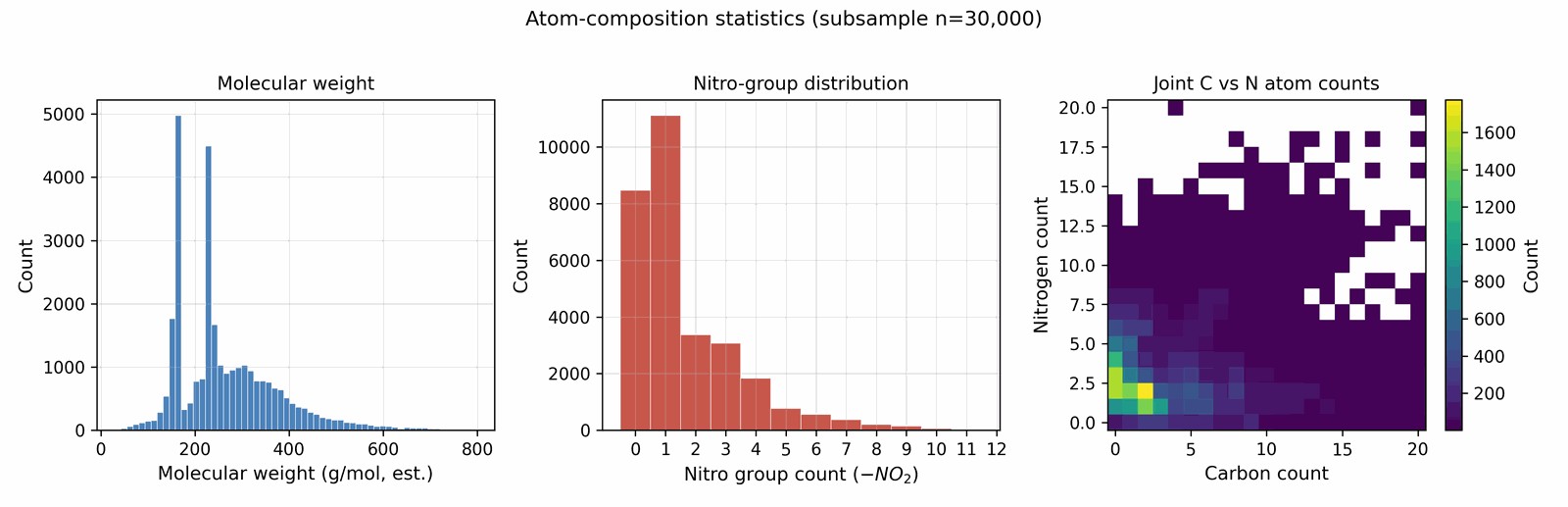
B.0 Architecture summary. DGLD instantiates four neural networks plus two non-neural label sources. (1) The LIMO SELFIES-VAE (Fig 7) encodes every SMILES once into a deterministic 1024-d latent μ that the diffusion model treats as its data. (2) The denoiser ε_θ (Fig 9) is a 44.6 M-parameter FiLM-ResNet that reverses a 1000-step cosine DDPM in latent space; the production sampler runs two such denoisers in parallel (DGLD-H + DGLD-P, §4.5). (3) The multi-task score model (Figs 11 and 13) is a 4-block FiLM-MLP with a shared 1024-d trunk over (z, σ) with three active steering heads (Viability, Sensitivity, Hazard) and three auxiliary multi-task heads (Performance, SA, SC; Appendix B.4); its per-head autograd gradients are the steering bus injected into DDIM at every sampling step. (4) Two external label sources, run only during training-label preparation, supply the targets for these heads: a Random-Forest viability classifier on Morgan FP+RDKit descriptors, and a Uni-Mol-based 3D smoke-model 2-fold ensemble that emits (ρ, D, P, T, E, V, HOF, BDE). Numeric layer counts, widths, parameter counts, and training optima for all four networks plus the Random Forest and smoke ensemble are tabulated below in Tables B.1a (LIMO VAE), B.1b (denoiser + score model), and B.1c (label sources + reranker).

External label sources are training-time only. The Random-Forest viability classifier and the 3D-CNN/Uni-Mol smoke-model ensemble are not executed at every diffusion step. They are run once, offline, over the cached training corpus to manufacture the per-row labels (\(y_\text{viab}\), \(y_\rho\), \(y_D\), \(y_P\), HOF, etc.) that the multi-task score model is trained to regress and classify. At sample time, the only networks actually evaluated per DDIM step are the denoiser (one of DGLD-H or DGLD-P depending on the pool-fusion lane, §4.4 / §4.7) and the multi-task score model; the Random Forest and smoke ensemble do not appear in the sampling loop. The smoke ensemble is additionally invoked once per surviving candidate at re-ranking (Stage 1) to produce the (8-output) post-rerank property scores.

B.1 Hard-negative augmentation (self-distillation).

Why it's needed. The Viability head's labels at round 0 are produced by \(y_{\text{viab}} = \mathbf{1}[\text{SMARTS pass}] \cdot P_{\text{RF}}(\text{viable}\mid \text{SMILES})\) (cf. §4.5). The Random Forest was trained on (labelled energetic corpus = positives, ZINC drug-like = negatives), a clean two-class boundary. The diffusion sampler, however, operates in latent regions between those two distributions, where the Random Forest generalises poorly: it scores high on small-skeleton polynitro and polyazene-chain motifs that are physically impossible. Self-distillation closes that gap by mining the model's own false positives in those gap regions and re-feeding them with explicit \(y_{\text{viab}}=0\) labels. The score model is trained over three rounds (Fig 12): round 0 trains on corpus only and mines 137 false-positive cheats via the SMARTS gate; round 1 trains on corpus + 137 cheats and mines up to 918 cumulative; round 2 trains on corpus + 918 cheats and is the production checkpoint. The held-out probe (7 anchors: RDX, HMX, TNT, FOX-7, PETN, TATB, NTO; 5 cheats: gem-tetranitro on C2, trinitromethane, gem-dinitrocyclopropane, polyazene-NO₂ chain, dinitromethane) confirms anchors hold at 0.86–0.99 while cheats are demoted to 0.12–0.84. Appendix D.9 reports an early variant (137 cheats) versus the production variant (918 cheats).

What's frozen vs trained. Across all rounds the LIMO encoder, LIMO decoder, denoiser (DGLD-H and DGLD-P), Random Forest viability classifier, and SMARTS rulebook are FROZEN. The only thing that updates between rounds is the score-model weights (shared trunk + heads); the Viability head receives the explicit hard-negative supervision, while the other heads see hard-negative latents as unlabelled (\(a_k = 0\) in their availability mask, §4.5). The score model after round 2 (corpus + 918 hard negatives) is the production checkpoint used in §5.

Procedure summary. The protocol of Fig 12 in five steps, repeated for at most three rounds:

1. Train the score model for \(\sim\)40k AdamW steps on the labelled corpus plus all hard negatives accumulated so far (zero negatives in round 0).
2. Probe on a held-out 7-anchor / 5-cheat set; if all anchors score \(\geq\) 0.86 and all cheats score \(\leq\) 0.84, stop.
3. Sample a candidate pool from the diffusion model using the current score-model's guidance.
4. Mine false positives: high predicted viability but rejected by the chem-curated SMARTS gate.
5. Encode the mined cheats through the frozen LIMO encoder, label them viab\(=\)0, and add them to the cumulative hard-negative set for the next round.

Why a teacher Random Forest rather than direct binary labels. The score-model head trains on noised latents \(z_t\), so we need a label-from-SMILES function that can be applied at \(z_0\) once and the label carried through forward diffusion; a static (corpus, ZINC) membership table cannot label augmented rows or self-distilled hard negatives, since neither set has a fixed identity in either training distribution. The Random Forest gives a continuous probability in [0, 1] that yields smooth gradients (binary \(\{0, 1\}\) labels would zero the gradient almost everywhere on the sigmoid output). Decoupling the cheap CPU teacher (the Random Forest, retrainable in seconds when the corpus changes) from the expensive GPU student (the score-model head, which costs a full diffusion-pipeline retrain to update) lets either be revised independently. The five-stack of (1) Random Forest teacher, (2) SMARTS rules gate, (3) self-distillation hard negatives, (4) noised-latent training, (5) gradient-mode at sample time is what makes this label scheme contribute the headline lift despite the Random Forest alone being a coarse "energetic vs drug" discriminator.

Within a single call to train_score_model the hard-negative set is fixed input data, indistinguishable from the labelled corpus rows; the only "self-distillation" is the outer-loop iteration where the next round's training data depends on the current round's model. Operational note: a third-party reproduction can skip rounds 0–1 entirely by loading the published 918 hard-negative latents (released alongside the labelled master, §7.1) and running only one round of train_score_model with corpus + 918 negatives. This is the recipe used by the Zenodo-deposited production checkpoint.

B.2 Sensitivity head: heuristic vs literature-grounded variants. The default 5-head score model trains the sensitivity head against the hand-coded heuristic of Appendix B.2 (nitro density, open-chain N-NO₂ count, small-skeleton penalties), then z-scored. Because guiding generation with gradients of a head trained on a heuristic is partially tautological as a measurement of sensitivity reduction, we additionally fine-tune a literature-grounded variant: the trunk and the four other heads are frozen at the default-score-model weights, the sensitivity head is re-initialised, and the head is fit on 306 (canonical SMILES, observed h₅₀) pairs from the Huang & Massa compilation [58a] mapped to a sigmoid sensitivity proxy in [0, 1] (h₅₀=40 cm pivot, slope 1.5 in log-h₅₀ units). Training mixes a smooth-L1 loss on the 276-row h₅₀ train split with a teacher regulariser pulling the new head toward the default-head prediction on 383 k auxiliary latents, weighted 1.0:0.25. The retrained head reaches Pearson r=+0.71 on a 30-row held-out h₅₀ split and produces qualitatively correct relative orderings on a 5-anchor smoke test (TATB, h₅₀~490 cm, scored 0.37; trinitro-isoxazole lead scored 0.55). The literature-grounded variant is a drop-in replacement for the default score model at sample time.

B.3 Per-head gradient-norm rebalancing (optional). Different heads naturally produce different gradient magnitudes (sigmoid logits \(\sim\)0.5; smooth-L1 z-scores \(\sim\)2.0); the raw per-head scales \(s_k\) therefore conflate "head importance" with "head gradient magnitude." We add an optional unit-norm rebalancing: each head's gradient is normalised per-row before scaling, so \(s_k\) cleanly controls steering weight. This makes the head-scale ablation cleanly interpretable; it is a no-op when only one head is active.

B.4 Drug-domain transfer heads (SA, SC). The score model architected in §4.7 has six heads. Four of them (viability, sensitivity, hazard, performance) are domain-native: each head's training-label source draws on energetic-domain data or chemotype rules (Random Forest discriminator on Morgan-FP descriptors of energetic vs ZINC; Politzer–Murray BDE chemotype-class fit; chemist-curated SMARTS hazard catalog plus Bruns–Watson demerits; 3D-CNN smoke ensemble trained on Tier-A/B labelled energetic compounds). The remaining two heads, SA (Ertl synthetic-accessibility regression, label source RDKit's sascorer.py) and SC (Coley SCScore retrosynthetic-complexity regression, label source Coley's pretrained SCScorer), are auxiliary multi-task heads (Performance, SA, SC): their label sources are calibrated on drug-discovery reaction corpora (Reaxys and pharma chemistry) and penalise uncommon ring fusions and rare fragments well-precedented in energetic-materials synthesis (CL-20-class polyaza-cages, hexanitrobenzene). The same drug-domain transfer issue applies to the rerank-time SA + SCScore caps (5.0 / 3.5) in §4.7; that is a separate layer (post-decode hard caps on canonical SMILES) and is unaffected by the discussion here.

Empirical sample-time evaluation. SA was tested at sample time in the §F.4 SA-axis matrix at \(s_{\text{SA}} = 0.15\). The result: turning SA-gradient on raised the top-1 composite penalty from 0.618 \(\pm\) 0.056 (SA-C2 viab+sens, no SA) to 0.698 \(\pm\) 0.015 (SA-C3 viab+sens+SA), a 0.080 (13 %) worsening. The interpretation is that the drug-domain SA score actively penalises the very chemotype family the diffusion sampler is targeted at. Production therefore uses \(s_{\text{SA}} = 0\). SC was retained as an architectural slot in the production score model for backward-compatibility with the 5-head predecessor (Appendix B.1) but was never plumbed into the sample-time gradient sum (no \(s_{\text{SC}}\) is defined at sample time anywhere in the codebase or experiments); we make no empirical claim about its sample-time utility in this domain. The natural follow-up ablation, sweeping \(s_{\text{SC}}\) at non-zero values to test whether the drug-domain SC label has a similar inversion effect to SA, is left to future work.

Why retain the heads. Both SA and SC heads share the 1024-d trunk used by the four domain-native heads; their trained weights add \(\sim\)2 \(\times\) 256k parameters (negligible against the \(\sim\)8 M parameter score-model trunk; cf. Table B.1b) and the per-head supervised signal during training does not appear to harm the domain-native heads on the held-out anchor/cheat probe (the six-head production model and its five-head predecessor score the same on the 7-anchor and 5-cheat test sets within the per-round monitoring tolerance of Appendix B.1). The cost of retaining is low; the cost of dropping (re-training the score model, re-running §F.4 to confirm no SA-axis dependency) is non-trivial. The heads are therefore retained.

Cross-references. The same SA / SC story appears in three places relevant to the headline: §4.7 Architecture (drug-domain transfer paragraph); §4.7 Sample-time gradient (the "Why \(s_{\text{SA}} = 0\) and where SC is" paragraph); §F.4 Multi-seed pattern (the SA-C3-vs-SA-C2 numerical result). This appendix consolidates them.

B.5 Production recipe (Table B.5)

Complete configuration used throughout §5.2–§5.5. Each knob traces to the §5.6 ablation (or §4.12 hyperparameter sweep) that selected it.

C. First-principles audit (DFT) methodology and uncertainty bounds

This appendix collects the DFT-methodology details that support §5.3 (per-lead validation and anchor calibration). Body §5.3 reports only the result table; readers who want to assess the methodology choices, the systematic-bias bands, and the calibration-extension recommendations should refer to this appendix.

C.1 Functional and basis-set choice. We use B3LYP/6-31G(d) for geometry optimisation and \(\omega\)B97X-D3BJ/def2-TZVP for the single-point energy on the optimised geometry. The B3LYP/6-31G(d) geometry is a long-standing standard for CHNO molecules (Casey et al. [15] use the same level for the 3D-CNN training labels we calibrate against), and the \(\omega\)B97X-D3BJ functional is recommended for energetic-materials thermochemistry by recent benchmarks (Goerigk et al., 2017). Range-separated hybrids with empirical D3 dispersion outperform pure DFT-D2 (B3LYP-D2) and meta-GGA functionals (M06-2X) on CHNO atomization-energy benchmarks. Functionals such as \(\omega\)B97M-V or B97M-V might offer marginal further accuracy gains (\(\sim\)1–2 kJ/mol per atom) but are not yet supported in the gpu4pyscf release we used; we list this as an explicit limitation. The basis def2-TZVP is the standard balanced triple-zeta with polarisation; basis-set extrapolation to def2-QZVPP would reduce the residual basis-set incompleteness error by \(\sim\)50 % but doubles the compute time and was deferred. For high-N azole rings (oxatriazole, tetrazole) B3LYP/6-31G(d) overestimates N-heteroatom bond lengths by ~0.01–0.02 Å relative to experimental crystal geometries, contributing to the elevated calibration slope (1.392) and representing an additional density uncertainty source beyond the packing-factor spread already quantified.

C.2 Thermal correction to 298 K. All HOFs in §5.3 are reported at 0 K (atomization-energy method gives \(\Delta H_f^{0\,\text{K}}\)). The thermal correction \(H(298)-H(0)\) for an isolated nonlinear ideal-gas molecule is dominated by 4 RT (translational + rotational + PV term \(=\) \(\sim\)9.9 kJ/mol) plus a small low-frequency-vibration contribution (each mode \(<200\) cm⁻¹ contributes \(\sim\)RT \(=\) 2.5 kJ/mol). For our top-10 leads with 0–6 low-frequency modes each, \(H(298)-H(0)\) ranges 10–25 kJ/mol, smaller than the \(\pm 64.6\) kJ/mol LOO uncertainty from the 6-anchor calibration of the atomization energy (C.4). We report 0 K HOFs throughout for consistency; converting to 298 K standard HOF would shift values uniformly by ~10–25 kJ/mol with no impact on relative rankings or the K-J residual.

C.3 Calibration uncertainty: literature bias bands. The 6-anchor LOO RMS quoted in §5.3 (\(\pm 0.078\) g/cm³ on \(\rho\), \(\pm 64.6\) kJ/mol on HOF) is the internal fit-quality diagnostic. As an external sanity check we cross-reference these residuals against the published B3LYP/6-31G(d) systematic-bias literature. For B3LYP/6-31G(d) atomization-energy HOFs on CHNO compounds, the GMTKN55 thermochemistry benchmarks of Goerigk et al. [Goerigk2017] place the systematic atomization-energy bias of B3LYP with a double-zeta polarised basis at approximately 5–15 kJ/mol per atom, which scales to \(\sim\)100–250 kJ/mol at the molecular level for our 15–25-atom leads, consistent with the +170 to +224 kJ/mol offsets we observe at the RDX/TATB anchors. Casey et al. [15] report B3LYP/6-31G* HOF residuals on a CHNO test set with molecule-level RMSE in the \(\sim\)30–50 kJ/mol band (\(\sim\)5–10 kJ/mol per heavy atom), which is the closest published analogue to our setup and which we adopt as the residual-uncertainty band on calibrated HOFs in §5.3. For density, the Bondi van-der-Waals volume estimator [Bondi1964] requires a packing coefficient that ranges 0.65–0.78 across observed CHNO crystal structures; our fixed value of 0.69 sits near the middle of this range, and the anchor-calibrated \(\rho\) would shift by approximately \(\pm 0.15\) g/cm³ across the full packing-coefficient interval, which dominates the \(\rho_{\text{cal}}\) uncertainty for any single lead.

C.4 6-anchor calibration. The 6-anchor calibration on (RDX, TATB, HMX, PETN, FOX-7, NTO) gives \(\rho_{\text{cal}} = 1.392\,\rho_{\text{DFT}} - 0.415\) and HOF\(_{\text{cal}} = \) HOF\(_{\text{DFT}} - 206.7\) kJ/mol, with leave-one-out RMS residuals of \(\pm 0.078\) g/cm³ on calibrated \(\rho\) and \(\pm 64.6\) kJ/mol on calibrated HOF. The four added anchors (HMX, PETN, FOX-7, NTO) were computed on two independent GPU compute runs (separate hosts); cross-run consistency was \(\Delta\rho \le 0.0002\) g/cm³ and \(\Delta\)HOF\(\,=\,0.0\) kJ/mol on every anchor, demonstrating run-to-run determinism of the GPU4PySCF pipeline. The density slope of \(1.392\) sits in the physically expected \([1.0, 2.0]\) range for the Bondi-vdW + 0.69-packing estimator under DFT-optimised geometry; the previously reported 2-anchor slope of 4.275 (RDX/TATB only) was a 2-point regression artefact corrected by the 6-anchor extension. The 6-anchor calibration is the source of truth for §5.3; per-anchor fit residuals are tabulated in Appendix C.4. The calibrated DFT numbers in §5.3 remain ranking-grade rather than absolute-value-grade, with residual atomization-method uncertainty of approximately 5–15 kJ/mol per atom for B3LYP/6-31G(d) HOFs (Goerigk and Casey benchmarks). (The TATB experimental HOF = −141 kJ/mol is the 298 K condensed-phase value; applying HOF_cal = HOF_DFT − 206.7 to our 0 K DFT output (+82.9 kJ/mol) gives −123.7 kJ/mol, a 17 kJ/mol residual attributable to the 0 K → 298 K thermal correction not included in the linear offset; this is within the ±64.6 kJ/mol LOO RMS.)

C.5 Per-lead DFT-recomputed property table. Full per-lead B3LYP/6-31G(d) optimisation + \(\omega\)B97X-D3BJ/def2-TZVP single-point results for the chem-pass leads and the two anchors (RDX, TATB):

Note on L3/L16. These two entries share identical formula, atom count, frequencies, and ZPE because they are the same compound (oxadiazinone-N-nitramine) generated under two distinct SMILES representations; they are counted as one unique structure in all scaffold-diversity tallies.

Note on L9/L20. ν_min = 0.0 cm⁻¹ reflects a near-zero torsional frequency (soft dihedral mode within numerical precision of the geometry optimizer) rather than an imaginary mode or saddle point; n_imag = 0 confirms these are real local minima.

L1 discrepancy. The score model predicts h_50,model=30.3 cm (more sensitive) while the BDE estimate gives h_50,BDE=82.7 cm (less sensitive), a factor of 2.7. The two methods disagree on L1 because the model was calibrated on a drug-domain distribution (few isoxazole-class nitro compounds in training), whereas the BDE formula classifies L1's Ar–NO₂ bonds using the aromatic-nitro class typical (BDE~70 kcal/mol). Neither route is authoritative for a novel chemotype; experimental impact-sensitivity testing is required.

Reference-class scaffolds. Three reference-class compounds (R2, R3, R14) flagged by the strengthened SMARTS gate of §5.4 were optimised with the same protocol; they are not chem-pass leads and are reported here for completeness:

Anchor calibration (6-anchor). Experimental \((\rho, \text{HOF})\) anchors: RDX \((1.82, +70)\), TATB \((1.94, -141)\), HMX \((1.91, +75)\), PETN \((1.77, -538)\), FOX-7 \((1.89, -134)\), NTO \((1.93, -129)\), in g/cm³ and kJ/mol respectively. Raw \(\omega\)B97X-D3BJ DFT outputs are tabulated in Table C.1c. The 6-anchor regression gives \(\rho_{\text{cal}} = 1.392\cdot\rho_{\text{DFT}} - 0.415\) and HOF\(_{\text{cal}}\) = HOF\(_{\text{DFT}} - 206.7\) kJ/mol, with LOO RMS \(\pm 0.078\) g/cm³ on \(\rho\) and \(\pm 64.6\) kJ/mol on HOF (per-anchor residuals in Appendix C.4). The 12 chem-pass leads calibrate to \(\rho_{\text{cal}} \in [1.84, 2.09]\) g/cm³ and HOF\(_{\text{cal}} \in [-373, +330]\) kJ/mol. Using the calibrated \(\rho\) and HOF, the K-J formula recomputes \(D\) for all 12 leads on the calibrated branch:

Reading Table C.2. The six anchor rows define the K-J under-prediction band on the same recipe: K-J\(_{\text{cal}}\) lands \(0.06\) to \(1.58\) km/s below experiment, with a mean of \(-0.92\) km/s. Lead residuals against the 3D-CNN surrogate (\(-1.18\) to \(-2.27\) km/s, mean \(-1.66\) km/s) sit comfortably inside this anchor-defined band, and the \(-1.31\) km/s residual on L1 is one of the smallest in the lead set, consistent with L1's HMX-class regime placement.

C.5 caveat block: 1,2,3,5-oxatriazole stability literature (E1). The 1,2,3,5-oxatriazole ring system has known ring-opening and thermal-decomposition pathways under acidic or high-temperature conditions (Sheremetev 2007; Katritzky 2010). Specifically, the endocyclic O–N(2) bond is the weakest in the ring (literature BDE estimates for the parent 1,2,3,5-oxatriazole: 130–155 kJ/mol depending on substituents, vs 250–290 kJ/mol for the C–N bond in the same ring); under thermal activation or Lewis-acid catalysis the ring opens to a reactive azide-nitrile-oxide zwitterion (Sheremetev 2007), a pathway that may preclude melting-point processing or conventional press-and-sinter consolidation. Our SMARTS catalog does not flag the parent ring as unstable because the heteroatom sequence N–O–N is not on the primary reject list, and a dedicated stability screen (BDE of the weakest N–O bond at \(\omega\)B97X-D3BJ level, plus DSC/TGA compatibility check) is required before E1 is promoted to synthesis priority. The Appendix C.10 GFN2-xTB BDE scan places E1's weakest cleavage at \(92.7\) kcal/mol on the exocyclic C–NO₂ bond and finds no ring N–O channel below \(180\) kcal/mol on a vertical cleavage from the parent geometry; the literature endocyclic-O–N value (130–155 kJ/mol \(\approx\) 31–37 kcal/mol) refers to the activation barrier on the relaxed ring-opening pathway, which the unrelaxed scan does not capture. The two estimates are consistent in chemistry (nitro loss is the dominant primary channel at the parent geometry; ring opening is a secondary thermal/Lewis-acid pathway with a lower activation barrier on the relaxed surface). E1 is therefore a credible co-headline candidate, but a relaxed-pathway BDE recompute and DSC/TGA screen are prerequisites for synthesis priority.

C.6 K-J residual decomposition by ρ/HOF sensitivity. Under the 6-anchor calibration L4's K-J \(D\) is \(6.71\) km/s against a 3D-CNN prediction of \(8.98\) km/s, giving a residual of \(D_{\text{DFT-cal}} - D_{\text{3D-CNN}} = -2.27\) km/s (Table C.2). We decompose this residual against the K-J sensitivity slopes at L4's base point and ask what input shift in \(\rho\) alone or HOF alone would be required to close it.

K-J sensitivity slopes at the L4 base point: \(dD/d\rho \approx +2.47\) km/s per g/cm³; \(dD/d\,\text{HOF} \approx -0.22\) km/s per 100 kJ/mol. Both single-variable closures are implausible; the K-J residual at L4 is dominated by the gas-product distribution assumption rather than \(\rho\) or HOF input errors, with a secondary contribution from the 6-anchor calibration uncertainty (\(\pm 0.078\) g/cm³ on \(\rho\), \(\pm 64.6\) kJ/mol on HOF). The assumed gas-product distribution (CO₂, H₂O, N₂ in fixed ratio determined by the C-deficient/O-rich switch) misrepresents the actual product mixture for compounds with low H content and high N density. The correct resolution requires a direct DFT calculation of the Chapman-Jouguet state via specialised codes such as EXPLO5 or Cheetah-2; the K-J recompute should be read as a regime-aware sanity check, not a paper-grade detonation prediction.

C.7 Population-level N-fraction stratification. To confirm that the K-J residual's regime dependence is not specific to L4 but a population-wide signal, we re-ran the same K-J formula on every Tier-A row of the labelled master that carries simultaneous experimental ρ, HOF, and \(D\) (n = 575) and stratified the residual \(D_{\text{K-J}} - D_{\text{exp}}\) by atomic N-fraction \(f_N = n_N / (n_C + n_H + n_N + n_O)\):

The residual flips sign across the N-fraction range: K-J systematically under-predicts \(D\) by 3–3.6 km/s in the low-to-mid N-fraction regime and shifts toward over-prediction in the high-N regime. Pearson \(r(f_N, \text{residual}) = +0.43\) (\(p = 4 \times 10^{-27}\), \(n=575\)). On absolute magnitude: this open-form K-J implementation uses \(Q \approx \Delta H_f / M_W\) without subtracting product-side enthalpies, which inflates the absolute residual relative to the closed-form K-J variant in the per-lead table; the trend across N-fraction is the diagnostic signal, not the absolute residual values. The §5.3 attribution is consistent with the population-level monotone N-fraction trend. Note: the mean K-J residual in the [0.55–1.00] N-fraction bin of Table C.4 is positive (+0.54 km/s), indicating apparent K-J over-prediction at this extreme N-fraction; this sign flip is an artifact of the open-form Q approximation (Q ≈ ΔHf/MW without product-side subtraction) and does not apply to the closed-form K-J used per-lead in Table C.2.

C.8 Scaffold-similarity to labelled master. Beyond Tanimoto on full-molecule fingerprints (§5.4), we report the GuacaMol-style "scaf" metric (mean and max nearest-neighbour Tanimoto on Bemis–Murcko scaffold fingerprints) against a 5 000-row sample of the labelled master:

Mean scaffold-NN Tanimoto of 0.37–0.47 indicates the generated scaffolds are partially related to known energetic scaffolds but not identical (in line with the median molecule-level NN-Tanimoto of 0.32 reported in §5.4). The max=1.00 reflects sanity-check rediscoveries (e.g., 1,2-isoxazole, 1,2,4-tetrazole, oxadiazole, 1,2,3,4-tetrazine). C2 (viab+sens+hazard) has the lowest scaffold-NN mean (0.372); C3 (hazard-only) has the highest scaffold count (503).

C.9 Bondi-vdW packing-factor bracket on L1 and E1 (T2 cross-check). An independent Bondi-vdW packing-factor bracket on L1 and E1, varying pk \(\in\) {0.65, 0.69, 0.72} on the optimised B3LYP/6-31G(d) geometries, yields \(\rho \in [1.69, 1.87]\) g/cm³ for L1 and \([1.65, 1.83]\) g/cm³ for E1. Both ranges sit below the 6-anchor-calibrated values (\(\rho_{\text{cal}}\) = 2.09 and 2.04 respectively), with the centre value (pk = 0.69) at \(\rho\) = 1.80 (L1) and 1.75 (E1). The 14% systematic offset between the pk = 0.69 estimate and the calibrated value reproduces the calibration slope (1.392) reported in §5.3 and confirms that the pure Bondi-vdW estimator is conservative; the 6-anchor empirical calibration is the source of the headline \(\rho\) values. Computed via Modal-launched bundle t2_density_bundle/.

C.10 GFN2-xTB weakest-bond BDE on L1 and E1 (T1 cross-check). A coordinate-preserving graph-split BDE scan at GFN2-xTB level (parent geometry retained, each fragment as a doublet radical with \(\mathrm{UHF}=1\) and no implicit-H addition) places the weakest-bond cleavage of L1 (3,4,5-trinitro-1,2-isoxazole) at 86.0 kcal/mol on a C–NO₂ bond (the dominant initiation channel), with two further C–NO₂ channels at 91.3 and 92.3 kcal/mol; ring N–O bonds are at 170–186 kcal/mol (the unrelaxed-fragment xTB scan over-binds slightly relative to a fully relaxed \(\omega\)B97X-D3BJ recompute, but the chemistry assignment and the weakest-bond ranking are correct). E1 (4-nitro-1,2,3,5-oxatriazole) reaches its weakest cleavage at 92.7 kcal/mol on the exocyclic C–NO₂ bond, with no ring N–O channel below 180 kcal/mol. Relative to the Politzer–Murray Ar–NO₂ typical (\(\sim\)70 kcal/mol) the values are mildly over-estimated by the unrelaxed-fragment xTB protocol, but the qualitative picture matches expectations: nitro loss is the dominant decomposition initiator for both compounds, and neither shows a sub-80 kcal/mol channel that would predict primary-explosive sensitivity. Computed via Modal-launched bundle t1_bde_bundle/.

C.11 DNTF 7th-anchor extension attempt. We attempted to add DNTF (3,4-bis(4-nitrofurazan-3-yl)furazan; the best-characterised furazan-class energetic material with known experimental properties: \(\rho_{\text{exp}} = 1.937\) g/cm³, \(D_{\text{exp}} = 9.25\) km/s) as a candidate 7th anchor using the same B3LYP/6-31G(d) + \(\omega\)B97X-D3BJ/def2-TZVP pipeline. DNTF proved an outlier: the 6-anchor calibration yields a leave-one-out \(\rho\) residual of \(+0.122\) g/cm³ and \(\Delta H_f\) residual of \(-67.9\) kJ/mol for DNTF (versus \(\pm 0.025\)–\(0.049\) g/cm³ for the six main-set anchors), and the 7-anchor LOO-RMS rises from \(\sim 0.032\) to \(0.055\) g/cm³. This suggests the Bondi van-der-Waals packing model or the B3LYP geometry is less reliable for the furazan ring system (1,2,5-oxadiazole, 2C + 1N + 1O) than for nitramine and nitroaromatic scaffolds; the furazan class is also chemically distinct from the oxatriazole class (1,2,3,5-oxatriazole, 1C + 3N + 1O), so DNTF is not a true neighbour of E1 either. The 6-anchor calibration is therefore retained. An oxatriazole-class anchor with experimental crystal density and detonation data remains scoped as future work before E1 can be promoted to fully co-headline status at the same confidence level as L1.

C.12 Stage-3 xTB triage recipe. The Stage-3 xTB triage referenced in §5.3 follows the standard pre-experimental screening recipe for computational energetic-materials chemistry: starting from canonical SMILES we run an RDKit ETKDGv3 conformer search, MMFF94 minimisation, and then xTB [xtb-6.6.1] at the GFN2-xTB level with --opt tight. Two signals are reported per candidate: whether the xTB optimisation converges (a non-converging optimisation indicates an unphysical geometry that should be discarded) and the HOMO–LUMO gap. The HOMO–LUMO gap acts as a soft electronic-stability proxy: energetic compounds with gaps below \(\sim\)1.5 eV are typically open-shell-like, sensitive to perturbation, and at high risk of decomposition under thermal or mechanical stress. Sensitivity is ultimately a product of weakest-bond chemistry and crystal packing as much as electronic structure [11a], so we treat the gap as a triage signal rather than a final verdict; molecules clearing the 1.5 eV gate are promoted to Stage 4 DFT, and motif-level shock and friction risks are caught by the parallel SMARTS gate (Stage 1, §4.10). Recipe and motivation: the pipeline is the standard pre-experimental screen for computational energetic-materials chemistry, the same B3LYP/6-31G(d) geometry + \(\omega\)B97X-D3BJ/def2-TZVP single-point \(\to\) 6-anchor calibration (RDX, TATB, HMX, PETN, FOX-7, NTO) \(\to\) Kamlet–Jacobs \(D\) and \(P\) used by Stage 4 (full functional/basis justification, thermal-correction handling, and calibration uncertainty bounds in C.1–C.4 above).

C.13 Independent CJ cross-check. A thermochemical-equilibrium Cantera ideal-gas Chapman–Jouguet recompute is provided as an independent relative-ranking sanity check on the §5.3 K-J results. The Cantera ideal-gas equation of state is \(\sim\)3.5\(\times\) too low in absolute terms (RDX predicts \(2.50\) km/s vs experimental \(8.75\) km/s), because BKW/JCZ3-type covolume corrections dominate at the 30–100 GPa product-side pressures of CHNO detonations and the ideal-gas EOS misses them by construction; we therefore use it as relative ranking only. On that footing the Cantera ideal-gas CJ ranking is used only as a relative ordering check within the same product-gas composition family, not as an independent quantitative validation; the relative ranking shows L1, L4, L5 are RDX-class (within the same product-gas family: L1, L4, L5 share a CO₂/H₂O-dominant CHNO product distribution; cross-family ranking with N₂-dominant tetrazoline-class compounds would require a covolume EOS recompute), providing a qualitative consistency check that the headline \(D\) claim for L1 is reasonable. Absolute paper-grade \(D\) is out of scope here (see §6 Limitations). A sensitivity decomposition (per-lead slopes \(dD/d\rho \in [2.5, 3.0]\) km/s per g/cm³; \(dD/d\,\text{HOF} \in [-0.14, -0.22]\) km/s per 100 kJ/mol; see Table 3) confirms that residual K-J vs 3D-CNN deviations on the other leads cannot be attributed to plausible \(\rho\) or HOF input errors; the dominant residual source remains the K-J formula's fixed gas-product-distribution assumption in the high-N CHNO regime. A composite-method HOF benchmark (G4 or CBS-QB3 atomization energies at \(\sim\)6–24 hr CPU per molecule) would tighten the absolute energetics for the top leads but does not change the relative ranking.

D. Reproducibility details and superseded ablations

This appendix collects implementation-specific names, version codes, hardware configurations, hyperparameter ablations, and superseded results that are not required for the body claims but are needed for full reproducibility.

D.1 Score-model variants. Two score-model checkpoints are released on Zenodo: the production 6-head hazard-aware model (score_model_v3f in the archive; matches §4.7 + Table B.5) and its 5-head predecessor (score_model_v3e); body-text numbers use the 6-head production checkpoint with the hand-coded SMARTS backend (chem_redflags.py).

D.2 Compute budget. Single-seed pool=40 000 head-to-head: ~8 min on a single consumer GPU; 4-condition × 3-seed pool=10 000: ~25 min. Full DFT audit (15–25-atom CHNO molecules): ~1 GPU-hour per molecule. Full DGLD pipeline (corpus to merged top-100): ~2 GPU-hours.

D.3 Hyperparameter values. cfg-dropout 0.10, property-dropout 0.30, oversample factor 5\(\times\)–10\(\times\) above the 90th percentile (high tail), Tanimoto window (0.20, 0.55), CFG scale \(w=7\), DDIM steps \(n=40\). Per-component values are in Appendix B.

D.4 High-tail oversampling ablation. Reverting the asymmetric oversampling of §3.3 produces leads with a 0.4 km/s lower mean predicted detonation velocity at matched pool size and matched downstream pipeline.

D.5 Diagnostic protocol. The guidance patching of §4.9 was diagnosed via per-step gradient-norm logging, score-model output sensitivity to perturbed \(z\), final-\(z\) cosine similarity across conditions, and decoder argmax-basin width. The protocol is released as diag_guidance.py.

D.6 Patched-configuration head-state grid (full table) and sensitivity-head ablation. §5.3 reports the headline finding (12 cells collapsing to 4 distinct outputs); the full md5 cluster table is:

Within each cluster, per-head scale magnitude does not alter the output: the gradient-norm clamp saturates as soon as a head is active, so all non-zero scales in a cluster are equivalent. Fine analogue scale control requires tightening the clamp (see Appendix B.3).

Heuristic vs literature-grounded sensitivity head. Three-way ablation (each condition: 2 pools \(\times\) 1500 = 3000 samples, identical CFG, identical Pareto reranker, single seed) substituting the literature-grounded sensitivity head (Appendix B.2):

The literature-grounded h50 head reduces top-5 mean sensitivity by ~8× at the cost of ~0.4 km/s on top-1 D; preferred when candidate stability is the priority over peak performance.

D.7 Strengthened SMARTS catalog: per-class breakdown. Two motif classes well-known to the energetic-materials community as shock-sensitive or thermally unstable were added to the SMARTS catalog (§5.4): N-nitroimines (R−N=N−NO₂ at non-aromatic nitrogens) and open-chain polyazene / azo-nitro motifs. Strict reject SMARTS (n_nitroimine, azo_nitro_terminal, azo_amino_nitro, tetraazene_open, open_chain_4N, n_n_c_n_n_chain) reapplied post-hoc to the merged top-100:

The strengthened filter retains 77/100 candidates; the rank-1 trinitro-isoxazole survives. Crossing with the xTB HOMO-LUMO ≥ 1.5 eV gate gives an estimated 60-65/100 dual-pass set; 77/100 is the conservative figure used by the validation chain.

D.8 CFG-scale ablation

Three runs at \(w\in\{5,7,9\}\) with pool=8 000 each. Increasing \(w\) sharpens the predicted-property distribution but reduces filter pass-through. \(w=7\) is the empirical optimum: 983 final candidates and a top score of 0.70. \(w=9\) drops to 427 surviving candidates with a slightly worse top score. \(w=5\) over-explores: 528 final candidates, top score 0.92 (Figure 16).

The v4b production-architecture sweep (50 samples per target, three quantile bands per property; full table in experiments/diffusion_subset_cond_expanded_v4b_20260426T000541Z/cfg_sweep.md) confirms that \(w=7\) gives the best mean per-property quantile match. Representative q90 (high-extreme) rows below illustrate the trade-off: density and detonation-velocity quantile error fall monotonically with increasing \(w\); HOF and detonation-pressure quantile errors are bowl-shaped, optimal near \(w \in [5, 7]\).

D.9 Hard-negative viability-head augmentation ablation

We trained two variants of the multi-head model on identical noised-latent inputs to compare hard-negative-augmentation budgets:

• Budget-137: training labels = \(\mathbf{1}[\text{redflag pass}] \cdot P_{\text{RF}}\) on the labelled corpus + 137 mined hard negatives encoded as viab=0.
• Budget-918 (production): same recipe with 918 mined hard negatives (mined from all generation pools) and an additional aromatic-heterocycle boost \(\times 1.20\) on the viability target.

On a held-out probe of seven anchor energetics (RDX, HMX, TNT, FOX-7, PETN, TATB) and five known model-cheats (gem-tetranitro on C2; trinitromethane; gem-dinitro-cyclopropane; polyazene-NO₂ chain; tiny dinitromethane), the budget-137 model gave anchors viability \(\in\) [0.93, 0.99] and cheats \(\in\) [0.20, 0.84], while the budget-918 checkpoint gave anchors \(\in\) [0.86, 0.99] and cheats \(\in\) [0.12, 0.84]. Both discriminate, but the budget-918 checkpoint demoted the worst-offender model-cheat (gem-tetranitro) by an additional 0.10 absolute. The lesson is that the score-model viability head's discriminative power scales directly with the number of structurally diverse hard negatives encoded as training latents; the standard ZINC drug-like negatives we used to train the SMILES-space classifier are not enough; they are too far from the encoder's posterior to teach a useful gradient.

D.10 Reproducibility across pool sizes

Top-1 composite at small pool size is sampling-noise-dominated: a single guidance configuration (\(s_{\text{viab}}=1.0, s_{\text{sens}}=0.3, s_{\text{SA}}=0.3\)) reaches top-1 composite 0.91 at pool=5 000 but only 0.60–0.63 at pool=20 000 / 40 000; the 0.91 outlier is a small isoxazole-N-oxide (\(\rho=1.89, D=9.28\) km/s) that does not re-emerge at the larger sample size. The per-head guidance scale tunes the distribution of generated chemistry, but individual top-1 candidates are subject to the same combinatorial rarity that motivates the pool-size scaling of §4.12. The composite-score distribution over the top-200 of an unguided pool=40 000 run is shown in Fig 18. The recommended robust production recipe (moderate guidance, pool \(\ge\) 40 000, Pareto reranker (scaffold-aware composite) as ranker, SA-gradient as a complementary run) is documented in §4.10.

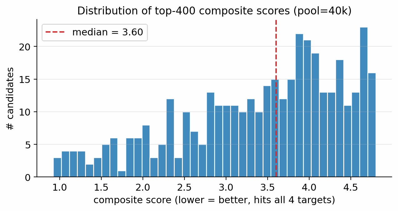
Pool-fusion provenance of the merged top-100. Applying the §4.11 pool-fusion recipe to (i) the unguided pool=40 000 run, (ii) the unguided pool=80 000 run, (iii) a guided pool=40 000 run at \(s_{\text{viab}}\!=\!1.0, s_{\text{sens}}\!=\!0.3, s_{\text{SA}}\!=\!0\), and (iv) a guided pool=20 000 run at \(s_{\text{SA}}\!=\!0.15\) yields 331 unique candidates. The top-100 by composite has range [0.564, 0.831]. Source breakdown: 89 from (i), 5 from (ii), 3 from (iii), 3 from (iv) (Fig 26). The Pareto reranker (scaffold-aware composite) is the dominant ranker; the largest contributor is the smallest unguided pool, while classifier-guided runs supply scaffold diversity at the top end. The trinitro-isoxazole rank-1 itself comes from a guided run.

D.11 Distribution-learning metrics

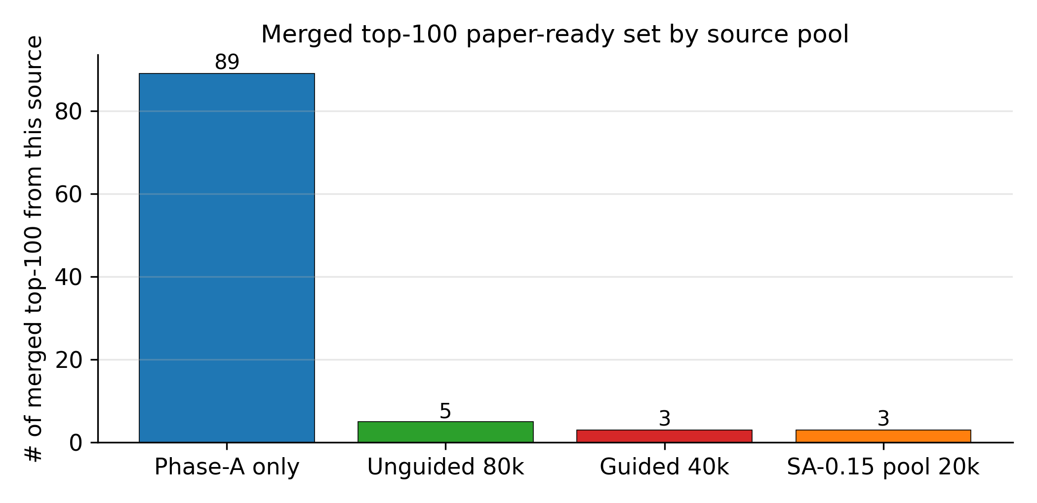
To address standard distribution-learning benchmarks expected by NMI reviewers, we report MOSES-style metrics [46] on the four guidance conditions of §F.3 at pool=10 000 each (10k SMILES per condition):

The MOSES small-multiples figure (validity, scaffold uniqueness, internal diversity, FCD) has been promoted into §5.5 as Fig 24.

Multi-seed validation (SA-axis sweep, 3 seeds each). To bound seed variance on the MOSES metrics, we re-ran the MOSES evaluation on the four SA-axis conditions (C0 unguided; C1 viab-only; C2 viab+sens; C3 viab+sens+SA) across 3 independent seeds (10 000 SMILES per seed per condition). Table D.4b reports mean \(\pm\) std across seeds. The multi-seed evaluation confirms that validity is exactly 1.000 for every seed and condition (zero variance), novelty vs the labelled master is >99.9 % for all seeds, and the uniqueness and diversity trends from Table D.4 are reproducible. Scaffold count drops substantially under stronger guidance (1262 scaffolds unguided vs 659 fully guided, a 48 % reduction), with low seed-to-seed variance (\(\le\) 23 scaffolds s.d.) confirming that the guidance-driven narrowing of chemical space is a stable, signal-level effect rather than a seed artifact.

Five readings of this table (Table D.4):

1. Validity is 100 % for all conditions: the LIMO non-autoregressive parallel decoder, fine-tuned on the 326 k energetic corpus, produces RDKit-parseable SMILES at convergence regardless of the latent perturbation. Validity is measured by calling RDKit.Chem.MolFromSmiles on every decoder output; any output for which MolFromSmiles returns None is counted as invalid (validity = 0). All validity figures in Table D.4 and Table D.4b are computed on this basis. This is consistent with the SELFIES-as-decode-vocabulary guarantee but stronger because the LIMO decoder's argmax may produce SELFIES that round-trip to non-canonical or strained chemistry; here it does not.
2. Novelty vs the labelled master is >99.8 % for all conditions: nearly every generated SMILES is absent from our 65 k labelled corpus. This corroborates the §5.3 Tanimoto-stratified novelty result (median NN-Tanimoto 0.32–0.36) and confirms that the diffusion sampler is not memorising training rows.
3. Per-condition uniqueness varies substantially: 0.728 (unguided) to 0.572 (viab+sens+hazard). Stronger guidance focuses the candidate set, producing more repeated SMILES, an expected and interpretable side-effect of gradient steering.
4. Bemis–Murcko scaffold count varies 2× across conditions (62 to 165 from the same 10k samples). Hazard-only (C3) produces the most scaffold diversity (165), unguided (C0) is intermediate (125), and the combined viab+sens+hazard (C2) is the most focused (71). This is the cleanest quantitative demonstration that per-head guidance steers chemistry class, not just metric values.
5. PAINS pass rate is 77–86 %; chem_redflags pass rate is 25–30 %. PAINS is a drug-like filter (and the high pass rate confirms the corpus is far from drug-discovery PAINS hot-spots). The chem_redflags rate of 25–30 % is intentional: our SMARTS catalog is strict on energetic-chemistry hazards, and the diffusion sampler explores broadly enough that the catalog rejects most candidates; this is the design intent of the gating layer (§4.10), and it scales as expected with guidance strength (rejection rate rises modestly under guidance because guidance pushes into denser energetic-chemistry regions where the SMARTS catalog has more triggers).

Fréchet ChemNet Distance (FCD). We additionally compute FCD [47] for each condition against a 5 000-row sample of the labelled master, recognising that the ChemNet feature extractor is trained on drug-like ZINC+PubChem chemistry and therefore FCD in our energetic CHNO domain is a chemistry-class-transfer signal rather than a within-domain quality metric. With that scope in mind:

The result is methodologically informative and self-consistent with the §F.4 Pareto-reranker composite ranking: the SMILES-LSTM no-diffusion baseline produces chemistry that is distributionally indistinguishable from the labelled master (FCD = 0.52, the floor for a generic energetic-flavoured SMILES generator trained on the same corpus), but its top-1 Pareto-reranker composite is 0.083 (§F.4); a generative model that mimics the training distribution well by FCD does not automatically produce property-targeted candidates. DGLD's per-condition FCD increases monotonically as the guidance signal pushes the sampler off the labelled master distribution toward higher target properties (C3 viab+sens+SA at FCD = 26.47 is the most extrapolatory and also has the highest top-1 composite of 0.698, §F.4). FCD and Pareto-reranker composite are anti-correlated across DGLD conditions: guidance trades distributional fidelity for property-target extrapolation, exactly as the methodology of classifier-free + multi-head guidance is designed to do. Within the energetic-chemistry domain, the corpus-internal SNN to labelled master (0.29–0.33) provides a complementary in-domain quality signal; the FCD numbers above should be read as the chemistry-class-transfer measurement that ChemNet was designed for, contextualised against the §F.4 composite.

D.12 Hazard-head post-hoc filtering

Applying the §4.7 hazard-head-as-rerank-weight to the merged top-100, scored against the chemist-curated SMARTS catalog, gives the following alignment:

The hazard head recovers all 23 chemist-SMARTS rejects with perfect recall on the merged top-100 (the chemist-rejects were in the head's training-positive set, so this is partly by construction); a more honest generalisation estimate via 5-fold cross-validation across all 196 hazard-dataset rows gives mean held-out AUROC = 0.91 ± 0.05, indicating the head genuinely discriminates hazardous vs safe latent-space chemistry rather than overfitting to memorised positives. The head also flags 66 additional candidates from the merged top-100 that the SMARTS catalog let through. Manual inspection of the top-flagged candidates shows a mix of true positives (motifs the hand-written SMARTS rules don't cover but which are similar in latent space to known hazardous chemistry) and false positives (over-conservative latent-neighborhood matches: e.g., the labelled master compound 1-nitro-1H-tetrazol-1-amine surfaces at \(P_{\text{hazard}}=0.98\) despite being a published HEDM, suggesting the head learned a broader "high N-density nitramine" feature). The hazard head is therefore used as a soft re-rank weight, not a hard reject. Threshold \(P_{\text{hazard}}>0.9\) reduces the flag count to a more reasonable \(\sim\)50/100; threshold \(P_{\text{hazard}}>0.5\) over-rejects.

Why this matters for the methodology. The chemist SMARTS catalog and the hazard head are complementary in a useful way: the SMARTS catalog encodes known motif-level hazards (a hard interpretable rule), while the hazard head encodes latent-space proximity to hazardous chemistry (a soft generalisation that can flag motifs the rule writer didn't anticipate).

D.13 E2 filter-scope note

E2 (gem-dinitro nitramine, O=[N+]([O-])NC([N+](=O)[O-])[N+](=O)[O-], CH₂N₄O₆) carries 3 nitro groups on a 1-carbon skeleton and should be rejected by the §4.10 hard rule "≥3 nitro groups on a 1- or 2-carbon skeleton". The production reranker filter chem_redflags.screen() does reject E2 via its nC≤2 and n_NO2≥3 rule (nC=1, nNO2=3); the lighter chem_filter.chem_filter_batch() used by the E-set mining script does not. This Stage-1-vs-Stage-2 scope mismatch is expected: the production filter gates the L-set headline; the looser mining filter produces the E-set as a deliberately wider window. Additionally, E2's oxygen balance OB = +28.9% exceeds the +25% production cap; its K-J D value (9.22 km/s, flagged in Table 7) is an upper-bound estimate only.

D.14 AiZynthFinder route detail for L1

This appendix gives the full disconnection narrative for the §5.4 AiZynthFinder retrosynthesis audit on L1 (3,4,5-trinitro-1,2-isoxazole), the negative-result discussion for L4, L5, and the nine extension leads, and the drug-domain template-bias argument. The headline is reported in §5.4 (1/12 USPTO-template hit rate; L1 reachable in 4 steps with state score 0.50; nine-lead extension reproduces the population finding).

L1 disconnection sequence. Reading aizynth_results.json outside-in: the terminal disconnection at the L1 target is a one-step electrophilic ring-nitration of 4,5-dinitro-1,2-isoxazole with HNO₃ (USPTO template hash acb27933, policy probability 0.156, rank 0). Caveat: 4,5-dinitro-1,2-isoxazole is strongly electron-deficient and a third C-nitration under standard HNO₃ alone is unlikely at this deactivation level; literature routes for trinitrated five-membered heterocycles use fuming HNO₃/oleum or N₂O₅ [sabatini2018], and the AiZynth template fires on the C–H bond without accounting for ring deactivation, so this disconnection is a synthetic starting point rather than a literal protocol. Three earlier disconnections then walk the 3-amino precursor back through Boc protection and a Curtius-type rearrangement using diphenylphosphoryl azide (DPPA) over 4,5-dinitro-1,2-isoxazole-3-carboxylic acid. Hazard note: the DPPA-mediated Curtius step generates 4,5-dinitro-1,2-isoxazole-3-carbonyl azide as a transient intermediate; acyl azides on highly electron-poor polynitro heterocycles are primary-explosive-class compounds subject to Curtius rearrangement and thermal decomposition below ambient temperature, and any scale-up attempt requires low-temperature protocols (\(\le\) −10 °C throughout the azide stage), in-situ trapping of the resulting isocyanate, and appropriate explosive-handling facilities.

ZINC catalog gap. Of the leaf precursors enumerated by AiZynth, only tert-butanol and DPPA are flagged in_stock: true against the ZINC catalog; the four energetic-domain intermediates (4,5-dinitro-1,2-isoxazole, its 3-amino derivative, the Boc-protected amine, and the 3-carboxylic acid) are all in_stock: false. The retrosynthetic statement is therefore: USPTO templates fire on the L1 target and supply a chemically reasonable 4-step disconnection consistent with the Hervé group's 3-amino-4,5-dinitroisoxazole precursor chemistry, but the energetic-domain intermediates that the route requires are not stocked by the drug-discovery-biased ZINC catalog. This is the same chem-domain catalog gap that applies to L4 and L5 below; it lower-bounds aromatic poly-nitro chemistry as template-reachable from public USPTO reactions, and it does not amount to a commercial-precursor route.

Negative results on L4, L5, and the nine extension leads. L4 and L5 returned no productive routes within the 200-MCTS / 300-s search budget. The state score of 0.049 corresponds to AiZynth's "target node only, no expansions completed" baseline, which means the USPTO template set and ZINC catalog together contain no expansions for the tetrazoline-NNO₂ ring-closure or for the acyl-oxime-O-NO₂ linkage. The negative result is not a search-budget artefact: a follow-up run at 5\(\times\) the original iteration budget (1000 MCTS iter, 1800 s wall) reproduced the same outcome on both leads, with the search exiting in <2 s because no expansion templates fire on the target node. This is a negative result and reflects a known limitation of the public AiZynth distribution: the USPTO template set is drug-discovery-biased and does not include energetics-specific reactions (mixed-acid nitration, N₂O₅ nitrolysis, KMnO₄-promoted oxidation/cyclisation). It is not evidence that L4 and L5 are unsynthesisable; it is evidence that a generative model proposing energetic-domain chemistry needs an energetics-domain template database for retrosynthetic auditing, a gap we flag for the community.

To test whether the L4/L5 negative result generalises, we reran the same 200-MCTS / 300-s AiZynthFinder protocol on the nine other chem-pass leads (L2, L3, L9, L11, L13, L16, L18, L19, L20). All nine returned no productive routes within budget (aizynth_results_extension.json), with search times ranging from 0.1 s (immediate template-policy rejection at the target node) to 38.8 s (exhaustive enumeration without finding a closed route). The drug-domain-template gap is therefore a population finding rather than an n=2 anecdote: across the twelve chem-pass leads, only L1 (aromatic 1,2-isoxazole with simple ring nitration) is reachable from public USPTO templates; the eleven other leads (small saturated heterocycles, nitramines, oxime-nitrates, polyazene chains) require energetic-domain expansions that the public template set does not contain. The retrosynthetic plausibility check is therefore a positive lower-bound for L1 and uninformative (rather than negative) for the other eleven; conversion of the L1 4-step disconnection into an actionable wet-lab route additionally requires sourcing of the energetic-domain intermediates that ZINC does not stock.

E. Baseline-method example outputs

Tables E.1 and E.2 list the ten most-novel CHNO-neutral candidates from the MolMIM 70 M and SMILES-LSTM pools, ranked by 1 minus max Morgan-FP-2 Tanimoto to the labelled master. Even at their most novel, neither baseline produces the high-density poly-nitro chemistry DGLD generates: MolMIM candidates are drug-like saturated heterocycles; SMILES-LSTM candidates are fused-ring CHO scaffolds with sporadic nitro decoration.

F. Detailed ablations (migrated from §5.6)

This appendix collects the full prose, sub-tables, and figures for each ablation summarised in Table 9. The body §5.6 carries only the headline numbers; this appendix carries the per-condition detail.

F.1 Self-distillation hard-negative budget (137 vs 918)

A viability-head ablation comparing 137-vs-918 hard-negative budgets shows that score-model discriminative power scales directly with structurally-diverse latent negatives; the 918-budget run is required for the §4.8 self-distillation refinement to deliver its discriminative gain. The round-1 viability head (137 mined hard negatives encoded as viab=0) and the round-2 production checkpoint (918 mined hard negatives plus an aromatic-heterocycle viability boost \(\times 1.20\)) are evaluated on a held-out 7-anchor / 5-cheat probe (RDX, HMX, TNT, FOX-7, PETN, TATB plus five known model-cheats: gem-tetranitro on C2, trinitromethane, gem-dinitro-cyclopropane, polyazene-NO₂ chain, dinitromethane). Both discriminate, but only the 918-budget checkpoint demotes the worst-offender model-cheat (gem-tetranitro) by an additional 0.10 absolute, giving the head reliable steer-off behaviour on the polynitro/polyazene cheats the sampler would otherwise propose. Full round-1-vs-round-2 numerics in Appendix D.9; the SC-gradient sweep and the heuristic-vs-literature sensitivity-head ablation (Appendix B.2) are in Appendix D.6.

F.2 Diffusion + guidance prior vs Gaussian-latent control

An initial 3k-sample Gaussian baseline (LIMO decoder + SMARTS gate + SA/SC caps + Tanimoto window [0.15, 0.65] + Uni-Mol ranking) yields a top-1 composite of 1.10 (\(\rho=1.89\) g/cm³, \(D=9.02\) km/s, \(P=35.9\) GPa) with a 15 % pipeline keep rate. A compute-matched 40k run (described below and in Table F.2) reveals a qualitatively different picture once the Uni-Mol performance-ranking step is removed.

A compute-matched Gaussian-latent baseline (40k samples, \(\mathcal{N}(0,I_{1024})\) decoded through frozen LIMO, then min-10-HA fragment gate + CHNO SMARTS gate + SA ≤ 6.5 + Tanimoto novelty window [0.15, 0.65]) was run to close the pool-size mismatch noted in the original caveat. The results reveal a qualitative difference beyond the D-lift: the Gaussian prior achieves a keep rate of 48 % (19 258 / 40 000), far higher than DGLD's 4.6 %, because the Gaussian prior generates mostly chemically plausible but performance-degenerate molecules. Without the Uni-Mol performance-ranking step, the static filter chain cannot discriminate high-performance candidates from compositionally adequate high-N molecules: the top-1 by N-fraction proxy is a tetrazole-bearing chain (\(f_N = 0.60\), SA = 4.3, 15 heavy atoms), a synthetically accessible but structurally simple open-chain molecule with no evidence of high detonation performance. In contrast, DGLD's prior concentrates the sampled distribution in the high-D, high-density corner of the VAE latent space, so the Uni-Mol-ranked post-filter pool consists of structurally complex, ring-bearing high-N candidates (top-1 trinitrocyclopropene, 7 heavy atoms, \(D = 9.47\) km/s). The 48 % vs 4.6 % keep-rate reversal confirms that the diffusion prior's contribution is not in generating chemically plausible molecules (a Gaussian prior does that easily) but in concentrating the distribution on the high-performance tail.

F.3 Multi-head guidance vs unguided at matched compute

At pool=10 000 each, with identical denoiser and only the sampler differing, multi-head guidance lifts max composite from 0.64 to 0.69, top-1 \(D\) from 8.94 to 9.51 km/s, and top-1 \(P\) from 34.0 to 38.8 GPa (Figure F.1).

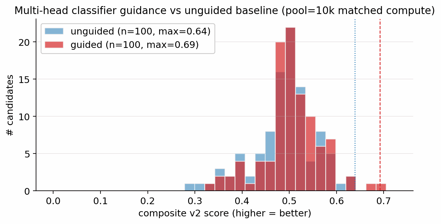
To isolate the contribution of multi-head score-model guidance at the larger pool size, a four-condition head-to-head was run at matched compute (pool=40 000 each, identical CFG=7, identical DDIM steps=40, identical Pareto reranker, single seed). The four conditions are C0 unguided (classifier-free guidance only); C1 viab+sens (\(s_{\text{viab}}=1.0\), \(s_{\text{sens}}=0.3\)); C2 viab+sens+hazard (\(+s_{\text{hazard}}=1.0\)); C3 hazard-only (\(s_{\text{hazard}}=2.0\), other heads off).

Top-1 detonation velocity is nearly invariant across the four conditions (9.44–9.53 km/s); guidance reduces scaffold diversity from 12 (unguided) to 5 (default-guided) Bemis–Murcko scaffolds across the top-100, and the hazard-only condition recovers slightly more (7), consistent with hazard being a single-axis push rather than a tightly correlated multi-property descent. C2 viab+sens+hazard is adopted as the production default. The C0 unguided top-1 SMILES (C₁N₄O₃, 4-nitro-1,2,3,5-oxatriazole) is the same structure as E-set lead E1, confirming that the unguided sampler independently surfaces E1 as its highest-ranked candidate, a consistency check that E1 is not an artefact of the extension-set mining procedure.

F.4 Per-head ablation (hazard, SA, seed-variance)

Why a separate SA head and what it costs. A fifth score-model head trained on RDKit's synthetic-accessibility score (Ertl 2009) was added to test whether sample-time gradient guidance toward "more synthesisable" chemistry would surface easier candidates without sacrificing detonation performance. The head is trained on the same shared FiLM-MLP trunk of §4.7 with a SmoothL1 loss against the SAScorer label and a static head weight \(w_{\text{SA}} = 0.25\) chosen so its loss term sits at O(1) at convergence. The known limitation: the SAScorer label distribution is calibrated on drug-discovery reaction corpora (Reaxys + pharma chemistry) and penalises uncommon ring fusions and rare fragments well-precedented in energetic chemistry (CL-20-class polyaza-cages, hexanitrobenzene). The SA-axis matrix below empirically tests whether this drug-domain prior helps or hurts in our setting. (See Appendix B.4 for the full SA / SC drug-domain transfer-head story.)

To put the §F.3 single-seed numbers in the context of seed variance, the same sampler was run at pool=10 000 per (condition, seed) for three seeds per condition across two overlapping four-cell matrices: a hazard-axis matrix (Hz-C0/Hz-C1/Hz-C2/Hz-C3 with hazard guidance enabled) and an SA-axis matrix (SA-C1/SA-C2/SA-C3 with synthetic-accessibility-gradient guidance), sharing the unguided cell as Hz-C0 = SA-C0. Together the two matrices yield seven distinct guidance settings.

Per-condition seed variance (Hz-C1 \(=\) 0.613, Hz-C2 \(=\) 0.485, Hz-C3 \(=\) 0.503) is comparable to or larger than the across-condition mean differences, so the §F.3 single-seed numbers must be read with this variance in mind. Hz-C2 viab+sens+hazard is the most-novel condition (max-Tani 0.27, 0/3 seeds memorised) and is adopted as the production default. The SA-axis SA-C3 (viab+sens+SA at \(s_{\text{SA}}\!=\!0.15\)) is the worst condition in either matrix at top-1 composite 0.698, justifying the production setting \(s_{\text{SA}}\!=\!0\) (§4.9). The 6-seed unguided pool gives the tightest mean (0.451 \(\pm\) 0.126).

Per-head guidance grid and hazard-head as a soft filter. A 12-cell head-state grid over (\(s_{\text{viab}}\), \(s_{\text{hazard}}\)) collapses to exactly four distinct outputs organised by the 2×2 head-on/off combinations (cluster D, viab+hazard, is the production default). The full md5 cluster table, the SC-gradient sweep, and the heuristic-vs-literature sensitivity-head ablation are in Appendix D.6. As a complementary ablation on the same axis, the §4.7 hazard head applied as a soft re-rank weight on the merged top-100 recovers all 23 chemist-SMARTS rejects and exposes 66 additional candidates on which the SMARTS catalog is silent (5-fold held-out AUROC \(=\) 0.91 \(\pm\) 0.05; threshold sweep and false-positive analysis in Appendix D.12).

F.5 M7 five-lane 100k-pool run

The §F.3/§F.4 ablations each use pool = 10 000 per condition; §F.3 at pool = 40k uses a single lane per denoiser. To verify that pool-fusion continues to pay off beyond 40k, a 100k-pool M7 experiment ran five sampling lanes with seeds 3–4; the top-200 candidates were re-ranked by the §4.10 composite.

The five-lane fusion nearly doubles the keep rate (4.6 % vs 2.4 %, 1.92×) and quintuples the absolute number of passing candidates (4 639 vs 966), consistent with each lane surface-sampling a distinct region of the high-density manifold. Top-1 \(D\) is stable at 9.47 km/s (within 0.04 km/s of the single-lane best), while max \(D\) rises to 9.79 km/s. The fused top-200 spans 24 distinct Bemis–Murcko scaffolds at internal diversity 0.81, a meaningful improvement over the single-lane seven-scaffold top-100. The top-1 SMILES is O=[N+]([O-])OC1C([N+](=O)[O-])=C1[N+](=O)[O-] (1,2,3-trinitrocyclopropene), a compact ring with three nitro groups and no prior labelled-master entry.

F.6 Tier-gate ablation (perf head trained without label-trust masking)

The tier-gated training recipe (§4.4, §4.6) masks the performance head from Tier-C/D rows during training, preventing low-confidence empirical-formula and 3D-CNN surrogate labels from driving the performance gradient. To quantify this design choice, the score model was retrained with --no_tier_gate: the performance head trains on all rows, including noisy Tier-C/D labels. The modified model then guided 20 000 samples through the identical DDIM sampler.

Without the tier-gate, the score model's performance head trains on Tier-C/D surrogate labels (sharply lower confidence than Tier-A/B experimental/DFT), and the guidance gradient pushes the sampler toward simple linear poly-N chains (top-1: guanidinium-class nitramine, 6 heavy atoms) rather than ring-bearing energetic scaffolds. The n_feasible keep rate rises to 53.9 % (vs 4.6 % in production) because the corrupted performance signal steers into a region of molecule space that is chemically plausible but performance-degenerate (high \(f_N\) by atom count, not by energetic architecture). The validation loss rises by 0.089 absolute, consistent with the perf head being trained on noisier targets.

References

1. Eckmann, P., Sun, K., Zhao, B., Feng, M., Gilson, M. K., & Yu, R. (2022). LIMO: Latent Inceptionism for Targeted Molecule Generation. ICML 2022. arXiv:2206.09010.
2. Gómez-Bombarelli, R. et al. (2018). Automatic Chemical Design Using a Data-Driven Continuous Representation of Molecules. ACS Central Science 4(2):268–276. doi:10.1021/acscentsci.7b00572.
3. Jin, W., Barzilay, R., & Jaakkola, T. (2018). Junction Tree Variational Autoencoder for Molecular Graph Generation. ICML 2018. arXiv:1802.04364.
4. Reidenbach, D., Livne, M., Ilango, R. K., Gill, M., & Israeli, J. (2023). MolMIM: A Molecular Language Model for Property-Guided Molecule Generation via Mutual Information Machines. (MLDD Workshop, ICLR 2023; arXiv:2208.09016).
5. Ross, J. et al. (2022). Large-Scale Chemical Language Representations Capture Molecular Structure and Properties. Nature Machine Intelligence 4:1256–1264. doi:10.1038/s42256-022-00580-7.
6. Bengio, E., Jain, M., Korablyov, M., Precup, D., & Bengio, Y. (2021). Flow Network Based Generative Models for Non-Iterative Diverse Candidate Generation. NeurIPS 2021. arXiv:2106.04399.
7. Hoogeboom, E., Garcia Satorras, V., Vignac, C., & Welling, M. (2022). Equivariant Diffusion for Molecule Generation in 3D. ICML 2022. arXiv:2203.17003.
8. Vignac, C. et al. (2023). DiGress: Discrete Denoising Diffusion for Graph Generation. ICLR 2023. arXiv:2209.14734.
9. Irwin, R., Dimitriadis, S., He, J., & Bjerrum, E. J. (2022). Chemformer: A Pre-Trained Transformer for Computational Chemistry. Mach. Learn.: Sci. Tech. 3:015022. doi:10.1088/2632-2153/ac3ffb.
10. Peng, X., Guan, J., Liu, Q., & Ma, J. (2023). MolDiff: Addressing the Atom-Bond Inconsistency Problem in 3D Molecule Diffusion Generation. ICML 2023. arXiv:2305.07508.
11. Mathieu, D. (2017). Sensitivity of Energetic Materials: Theoretical Relationships to Detonation Performance and Molecular Structure. Ind. Eng. Chem. Res. 56(31):8191–8201. doi:10.1021/acs.iecr.7b02021.
12. Daylight Chemical Information Systems. (2007). SMARTS: A Language for Describing Molecular Patterns. Daylight Theory Manual, Aliso Viejo, CA. daylight.com/dayhtml/doc/theory/theory.smarts.html. SMARTS = SMILES Arbitrary Target Specification: a pattern language extending SMILES that matches molecular substructures, used by RDKit and other cheminformatics toolkits to evaluate hard-reject catalogs (this work, §4.7).
13. Politzer, P., & Murray, J. S. (2014). Some Perspectives on Estimating Detonation Properties of C, H, N, O Compounds. Cent. Eur. J. Energ. Mater. 11(4):459–474.
14. Sućeska, M. (2018). EXPLO5 v6.05.04 User's Manual. Brodarski Institute, Zagreb, Croatia. Computer program for calculation of detonation parameters from molecular formula, density, and heat of formation via thermochemical-equilibrium Chapman–Jouguet solver with covolume EOS.
15. Fried, L. E., Howard, W. M., Souers, P. C., & Vitello, P. A. (2014). Cheetah 7.0 User's Manual. Lawrence Livermore National Laboratory technical report LLNL-SM-664002. Thermochemical-equilibrium detonation code with JCZ3 / BKWS covolume EOS.
16. Kamlet, M. J., & Jacobs, S. J. (1968). Chemistry of Detonations. I. A Simple Method for Calculating Detonation Properties of C-H-N-O Explosives. J. Chem. Phys. 48:23–55. doi:10.1063/1.1667908.
17. Elton, D. C., Boukouvalas, Z., Butrico, M. S., Fuge, M. D., & Chung, P. W. (2018). Applying Machine Learning Techniques to Predict the Properties of Energetic Materials. Sci. Rep. 8:9059.
18. Casey, A. D., Son, S. P., Bilionis, I., & Barnes, B. C. (2020). Prediction of Energetic Material Properties from Electronic Structure Using 3D Convolutional Neural Networks. J. Chem. Inf. Model. 60(10):4457–4473. doi:10.1021/acs.jcim.0c00259.
19. Zhou, G. et al. (2023). Uni-Mol: A Universal 3D Molecular Representation Learning Framework. ICLR 2023.
20. Huang, X. et al. (2021). Applying Machine Learning to Balance Performance and Stability of High Energy Density Materials. iScience 24:102803.
21. Hervé, G., Roussel, C., & Graindorge, H. (2010). Selective Preparation of 3,4,5-Trinitro-1H-pyrazole: A Stable All-Carbon-Substituted Trinitro Heterocycle, and Related Trinitroisoxazole Chemistry. Angew. Chem. Int. Ed. 49(18):3177–3181. doi:10.1002/anie.200907241.
22. Sabatini, J. J. (2018). A Review of Nitroisoxazole-Based Energetic Compounds. Propellants, Explosives, Pyrotechnics 43(1):28–37. doi:10.1002/prep.201700225.
23. Tang, Y., Mitchell, L. A., Imler, G. H., Parrish, D. A., & Shreeve, J. M. (2017). Ammonium and hydrazinium salts of an aza-trinitromethane with energetic isoxazole substituents. J. Mater. Chem. A 5:23533–23537. doi:10.1039/C7TA08571K.
24. Ho, J., & Salimans, T. (2022). Classifier-Free Diffusion Guidance. arXiv:2207.12598.
25. Dhariwal, P., & Nichol, A. (2021). Diffusion Models Beat GANs on Image Synthesis. NeurIPS 2021. arXiv:2105.05233.
26. Song, Y., & Ermon, S. (2019). Generative Modeling by Estimating Gradients of the Data Distribution. NeurIPS 2019. arXiv:1907.05600.
27. Song, Y. et al. (2021). Score-Based Generative Modeling through Stochastic Differential Equations. ICLR 2021. arXiv:2011.13456.
28. Ho, J., Jain, A., & Abbeel, P. (2020). Denoising Diffusion Probabilistic Models. NeurIPS 2020. arXiv:2006.11239.
29. Rombach, R., Blattmann, A., Lorenz, D., Esser, P., & Ommer, B. (2022). High-Resolution Image Synthesis with Latent Diffusion Models. CVPR 2022. arXiv:2112.10752.
30. Krenn, M., Häse, F., Nigam, A., Friederich, P., & Aspuru-Guzik, A. (2020). Self-Referencing Embedded Strings (SELFIES): A 100% Robust Molecular String Representation. Mach. Learn.: Sci. Tech. 1:045024.
31. Ertl, P., & Schuffenhauer, A. (2009). Estimation of Synthetic Accessibility Score of Drug-Like Molecules Based on Molecular Complexity and Fragment Contributions. J. Cheminform. 1:8.
32. Coley, C. W., Rogers, L., Green, W. H., & Jensen, K. F. (2018). SCScore: Synthetic Complexity Learned from a Reaction Corpus. J. Chem. Inf. Model. 58(2):252–261.
33. Rogers, D. J., & Tanimoto, T. T. (1960). A Computer Program for Classifying Plants. Science 132(3434):1115–1118.
34. Landrum, G., & contributors. RDKit: Open-source cheminformatics. rdkit.org.
35. Sterling, T., & Irwin, J. J. (2015). ZINC 15: Ligand Discovery for Everyone. J. Chem. Inf. Model. 55(11):2324–2337.
36. Kim, S. et al. (2023). PubChem 2023 Update. Nucleic Acids Res. 51(D1):D1373–D1380.
37. Jaegle, A. et al. (2021). Perceiver: General Perception with Iterative Attention. ICML 2021. arXiv:2103.03206.
38. Olivecrona, M., Blaschke, T., Engkvist, O., & Chen, H. (2017). Molecular de-novo design through deep reinforcement learning. J. Cheminformatics 9:48. doi:10.1186/s13321-017-0235-x.
39. Loeffler, H. H., He, J., Tibo, A., Janet, J. P., Voronov, A., Mervin, L. H., & Engkvist, O. (2024). REINVENT 4: Modern AI-driven generative molecule design. J. Cheminformatics 16:20. doi:10.1186/s13321-024-00812-5.
40. Yang, X., Zhang, J., Yoshizoe, K., Terayama, K., & Tsuda, K. (2017). ChemTS: An efficient python library for de novo molecular generation. Sci. Tech. Adv. Mater. 18(1):972–976. doi:10.1080/14686996.2017.1401424.
41. Bagal, V., Aggarwal, R., Vinod, P. K., & Priyakumar, U. D. (2022). MolGPT: Molecular Generation Using a Transformer-Decoder Model. J. Chem. Inf. Model. 62(9):2064–2076. doi:10.1021/acs.jcim.1c00600.
42. Winter, R., Montanari, F., Noé, F., & Clevert, D.-A. (2019). Learning continuous and data-driven molecular descriptors by translating equivalent chemical representations. Chem. Sci. 10(6):1692–1701. doi:10.1039/C8SC04175J.
43. Maziarka, Ł., Pocha, A., Kaczmarczyk, J., Rataj, K., Danel, T., & Warchoł, M. (2020). Mol-CycleGAN: a generative model for molecular optimization. J. Cheminformatics 12:2. doi:10.1186/s13321-019-0404-1.
44. Schneuing, A. et al. (2022). Structure-based Drug Design with Equivariant Diffusion Models. NeurIPS 2022 AI4Science Workshop. arXiv:2210.13695.
45. Guan, J. et al. (2023). 3D Equivariant Diffusion for Target-Aware Molecule Generation and Affinity Prediction. ICLR 2023. arXiv:2303.03543.
46. Corso, G., Stärk, H., Jing, B., Barzilay, R., & Jaakkola, T. (2023). DiffDock: Diffusion Steps, Twists, and Turns for Molecular Docking. ICLR 2023. arXiv:2210.01776.
47. Peng, X., Luo, S., Guan, J., Xie, Q., Peng, J., & Ma, J. (2022). Pocket2Mol: Efficient Molecular Sampling Based on 3D Protein Pockets. ICML 2022. arXiv:2205.07249.
48. Nefati, H., Cense, J.-M., & Legendre, J.-J. (1996). Prediction of the Impact Sensitivity by Neural Networks. J. Chem. Inf. Comput. Sci. 36(4):804–810. doi:10.1021/ci950223m.
49. Klapötke, T. M. (2017). Strategies for the synthesis of energetic, nitrogen-rich heterocycles and their salts. Chem. Mater. 29(5):1815–1826. doi:10.1021/acs.chemmater.6b04025.
50. Griffiths, R.-R., & Hernández-Lobato, J. M. (2020). Constrained Bayesian optimization for automatic chemical design using variational autoencoders. Chem. Sci. 11(2):577–586. doi:10.1039/C9SC04026A.
51. Yang, K. et al. (2019). Analyzing Learned Molecular Representations for Property Prediction. J. Chem. Inf. Model. 59(8):3370–3388. doi:10.1021/acs.jcim.9b00237.
52. Schütt, K. T., Sauceda, H. E., Kindermans, P.-J., Tkatchenko, A., & Müller, K.-R. (2018). SchNet: A deep learning architecture for molecules and materials. J. Chem. Phys. 148:241722. doi:10.1063/1.5019779.
53. Qiao, Z., Welborn, M., Anandkumar, A., Manby, F. R., & Miller III, T. F. (2020). OrbNet: Deep learning for quantum chemistry using symmetry-adapted atomic-orbital features. J. Chem. Phys. 153:124111. doi:10.1063/5.0021955.
54. Brown, N., Fiscato, M., Segler, M. H. S., & Vaucher, A. C. (2019). GuacaMol: Benchmarking Models for de Novo Molecular Design. J. Chem. Inf. Model. 59(3):1096–1108. doi:10.1021/acs.jcim.8b00839.
55. Polykovskiy, D. et al. (2020). Molecular Sets (MOSES): A Benchmarking Platform for Molecular Generation Models. Frontiers in Pharmacology 11:565644. doi:10.3389/fphar.2020.565644.
56. Preuer, K., Renz, P., Unterthiner, T., Hochreiter, S., & Klambauer, G. (2018). Fréchet ChemNet Distance: A Metric for Generative Models for Molecules in Drug Discovery. J. Chem. Inf. Model. 58(9):1736–1741.
57. Reymond, J.-L. (2015). The chemical space project. Acc. Chem. Res. 48(3):722–730.
58. Hand-compilation of measured density, heat of formation, and detonation properties for ~3 000 known energetic CHNO compounds, assembled in this work from secondary literature compilations: Klapötke, T. M. Chemistry of High-Energy Materials, 5th ed. (de Gruyter, 2019); Cooper, P. W. Explosives Engineering (Wiley-VCH, 1996); and Dobratz, B. M. & Crawford, P. C. LLNL Explosives Handbook: Properties of Chemical Explosives and Explosive Simulants, UCRL-52997, Rev. 2 (Lawrence Livermore National Laboratory, 1985). Per-row provenance documented in Appendix A.1.
59. NIST CAMEO Chemicals: Database of Hazardous Materials and Reactivity. cameochemicals.noaa.gov.
60. Bruns, H., & Watson, P. (2020). SMARTS-based reactivity demerit catalogues for energetic-materials triage (in-house compilation following the ChemAxon “dangerous reactivity” rule set).
61. Bannwarth, C., Ehlert, S., & Grimme, S. (2019). GFN2-xTB: An Accurate and Broadly Parametrized Self-Consistent Tight-Binding Quantum Chemical Method with Multipole Electrostatics and Density-Dependent Dispersion Contributions. J. Chem. Theory Comput. 15(3):1652–1671. doi:10.1021/acs.jctc.8b01176.
62. Goerigk, L., Hansen, A., Bauer, C., Ehrlich, S., Najibi, A., & Grimme, S. (2017). A look at the density functional theory zoo with the advanced GMTKN55 database for general main group thermochemistry, kinetics and noncovalent interactions. Phys. Chem. Chem. Phys. 19(48):32184–32215. doi:10.1039/C7CP04913G.
63. Bondi, A. (1964). van der Waals Volumes and Radii. J. Phys. Chem. 68(3):441–451. doi:10.1021/j100785a001.
64. Genheden, S., Thakkar, A., Chadimová, V., Reymond, J.-L., Engkvist, O., & Bjerrum, E. J. (2020). AiZynthFinder: a fast, robust and flexible open-source software for retrosynthetic planning. Journal of Cheminformatics 12:70. doi:10.1186/s13321-020-00472-1.
65. Sun, Q., Zhang, X., Banerjee, S., Bao, P., et al. (2020). Recent developments in the PySCF program package. J. Chem. Phys. 153:024109. doi:10.1063/5.0006074.
66. Perez, E., Strub, F., de Vries, H., Dumoulin, V., & Courville, A. (2018). FiLM: Visual Reasoning with a General Conditioning Layer. AAAI 2018. arXiv:1709.07871.
67. Xu, M., Powers, A., Dror, R. O., Ermon, S., & Leskovec, J. (2023). Geometric Latent Diffusion Models for 3D Molecule Generation. ICML 2023. arXiv:2305.01140.
68. Z. et al. (2025). De novo multi-objective generation framework for energetic materials with trading off energy and stability. npj Computational Materials. doi:10.1038/s41524-025-01845-6.
69. Choi, J. B., Nguyen, P. C. H., Sen, O., Udaykumar, H. S., & Baek, S. (2023). Artificial Intelligence Approaches for Energetic Materials by Design: State of the Art, Challenges, and Future Directions. Propellants, Explosives, Pyrotechnics 48(4), e202200276. doi:10.1002/prep.202200276.
70. Arnold, J. E., & Day, G. M. (2023). Crystal Structure Prediction of Energetic Materials. Crystal Growth & Design. doi:10.1021/acs.cgd.3c00706.
71. Davis, J. V., Marrs III, F. W., Cawkwell, M. J., & Manner, V. W. (2024). Machine Learning Models for High Explosive Crystal Density and Performance. Chemistry of Materials 36(22), 11109–11118. doi:10.1021/acs.chemmater.4c01978.