Anomaly Detector Model Selection by Normal Manifold Separability

1. Introduction

Deploying an anomaly detector on a new dataset without labeled anomalies is common in fraud, industrial monitoring, health, and cybersecurity. The best detector for a given problem is not known in advance and varies widely across datasets. Isolation Forest wins on some datasets, LOF on others, ECOD on yet others. Without labels, the practitioner picks by prior, by convenience, or by expensive human review. Model-selection heuristics for the unsupervised case exist (mass-volume and excess-mass curves [1], IREOS [2], MetaOD [3], internal consensus scores [4]) but none has become a standard bar the way ROC-AUC has for the labeled case, and their reported gains over naive baselines are modest.

We ask a simpler question: if we cluster the unlabeled data and treat a small cluster as if it were an anomaly cluster, does the ranking of detectors on this pseudo-anomaly task predict the ranking on real anomalies? The intuition runs through the detector's competence. Every anomaly detector is at heart a model of where the normal data lies, and it flags whatever falls outside that model, so a detector is only as good as its grasp of the normal geometry. A detector that has genuinely captured that geometry should recognize any coherent group of points that sits apart from the bulk, including a held-out cluster we designate as a stand-in anomaly. How well it separates that held-out cluster from the rest of the normal data is therefore a readout of how well it has modeled normal structure, the same competence it needs to separate true anomalies from normal. We can then rank detectors by their average pseudo-AUC across many cluster-holdout draws, without ever seeing a label. The reading is faithful to the degree that real anomalies resemble held-out clusters, compact and locally distinct, which is where the method works and, where they do not, where it meets its ceiling.

Our contributions:

1. NoMaS, an unsupervised ranking procedure for anomaly detectors. Cluster once, hold out subsets of clusters as pseudo-anomalies, fit each detector on the complement, aggregate pseudo-AUC across draws.
2. A regret-based evaluation of unsupervised detector selection that is threshold-free and stable, avoiding the boundary artifacts of thresholded rank-correlation, and an empirical validation on 69 datasets across four modalities (tabular, image, text, time-series) with 9 canonical PyOD detectors and five seeds. NoMaS cuts selection regret versus random by 73-90% on all four. The natural consensus baseline scores Spearman ρ = -0.15, worse than random.
3. An unsupervised auto-calibration that recovers near-oracle regret on every modality: run a bank of pseudo-anomaly regimes and weight each by its cross-detector pseudo-AUC variance, a label-free measure of how informative the regime is. This weighting reaches 78-93% below random on all four modalities and cuts regret on the two embedding modalities a further 2-4× (text from 0.022 to 0.006), because it automatically up-weights a locally-embedded ("hard") regime that exercises the local-density structure embedding detectors need.
4. A selector that is trustworthy on two axes practitioners care about. The ranking signal comes from normal-data geometry alone: regret is flat as real anomalies are added to the unlabeled input and unchanged at 0% contamination (pure normals). And against the demanding baseline of a single fixed detector, NoMaS has the lowest mean regret of any label-free strategy, beating the Isolation Forest default (paired p < 0.05 on image, text, and tabular; p < 0.001 on the two embedding modalities) and matching the best fixed detector without knowing which one it is, both in-distribution and on 187 previously-unseen OddBench datasets.
5. Ablations, panel robustness, and stability analyses: the hand-designed composite "anomaly-likeness" selector we expected to help was the worst of three; leave-one-detector-out never materially changes the ranking; and calibrated regret is stable across seeds (std ≤ 0.002).

2. Related work

Anomaly detectors and benchmarks. Established detectors span the standard families: isolation-based (Isolation Forest [8]), density-based (LOF [9]), boundary-based (one-class SVM [10]), distribution-based (COPOD [11], ECOD [12]), projection-based (LODA [13], PCA), and deep one-class methods (DeepSVDD [14]). Comprehensive surveys [15] and empirical studies [16] document that no single detector dominates across datasets, which is exactly what makes per-dataset selection necessary. Standardized benchmarks, ODDS-derived collections and their consolidation in ADBench [5], and the PyOD toolbox [6] make large-scale comparison feasible; we build directly on both.

Unsupervised model and hyperparameter selection. The central difficulty is choosing among detectors or configurations without labels. Internal metrics score a single detector from properties of its own output: excess-mass and mass-volume curves [1], and the internal relative-evaluation score IREOS [2]. These are detector-anchored and do not define a common task on which two detectors are directly comparable. Meta-learning approaches such as MetaOD [3] regress from dataset meta-features to expected performance, but require a labeled meta-training corpus and generalize only within its coverage. A recent review [17] evaluates a broad set of internal strategies and finds that none is reliably better than naive baselines across benchmarks, motivating fundamentally different signals. NoMaS instead constructs a common pseudo-labeled task per dataset and lets ROC-AUC rank the detectors, needing neither labels nor meta-training.

Consensus and outlier ensembles. Averaging or combining detector scores yields a consensus outlier score used both as an ensemble output and, implicitly, as a selection signal that favors detectors agreeing with the majority [4, 18]. Our experiments show consensus fails as a ranking signal on ADBench (ρ = -0.15): the detectors most correlated with the panel mean are not those most correct on real anomalies. NoMaS does not assume agreement implies correctness; it measures each detector against an externally constructed pseudo-labeled task.

Pseudo-labels and self-supervised anomaly detection. Synthetic-anomaly injection is standard for turning unsupervised detection into a discriminative problem, and its effectiveness depends heavily on how realistic the injected anomalies are [7]. Self-supervised methods create surrogate tasks, geometric-transformation prediction [19] or learned classification pretexts [20], whose auxiliary loss serves as an anomaly score. All of these use pseudo-labels to train a single detector. NoMaS uses pseudo-labels for the different purpose of ranking a panel: the pseudo-anomalies (held-out clusters) need not resemble real anomalies well enough to train a detector, only well enough to order detectors by difficulty.

3. Method

A detector that understands normal data well enough to tell its own sub-structure apart should, for the same reason, tell normal from anomalous; we measure the first to predict the second.

Let $X \in \mathbb{R}^{n \times d}$ be an unlabeled tabular dataset and let $\mathcal{D} = \{D_1, \dots, D_L\}$ be a panel of anomaly detectors. Each detector produces a decision function $s_D: \mathbb{R}^d \to \mathbb{R}$ where higher values mean more anomalous. Our goal is a per-dataset ranking $\pi_X: \mathcal{D} \to \{1, \dots, L\}$ that approximates the ranking $\pi_X^*$ induced by ROC-AUC on real anomaly labels.

Embedding and clustering. Standardize $X$ and apply PCA to 16 dimensions (or keep $d$ if $d \le 16$). Cluster the embedding with MiniBatchKMeans at $K$ clusters, obtaining assignments $\ell : \{1, \dots, n\} \to \{1, \dots, K\}$.

Cluster subset sampling. Rank clusters by size ascending and let the candidate pool $\mathcal{C}$ be the smallest half. For each of $M = 20$ draws, sample from $\mathcal{C}$ without replacement until the union has size $\ge \max(20, 0.05 n)$. The union $S_j$ is the pseudo-anomaly set for draw $j$. From the complement, uniformly sample 20% as the pseudo-normal fold $N_j$; the remainder is the training set $T_j$.

Held-out-cluster separability. For each detector $D$ and draw $j$, fit $D$ on $T_j$, score both $S_j$ and $N_j$, and compute the pseudo-AUC $A_{D,j} = \mathrm{AUC}(\mathbf{1}_{S_j}, s_D)$ with $S_j$ labeled 1 and $N_j$ labeled 0. This pseudo-AUC is the detector's held-out-cluster separability: how well its scores pull the excised cluster $S_j$ apart from the retained normals $N_j$. If $D$ fails on $T_j$, or emits a non-finite or constant score vector, set $A_{D,j}$ to missing.

Aggregation and ranking. Within one regime, the aggregation is $\bar A_D = \operatorname{mean}_j A_{D,j}$ over non-missing $j$, our estimate of detector $D$'s normal-manifold separability, and detectors are ranked by $\bar A_D$ descending. Borda over per-draw ranks and variance-weighted mean perform within ±0.02 ρ of the mean.

Auto-calibration over a regime bank. A single pseudo-anomaly regime (one cluster-selection rule and one $K$) can be blind to the structure that separates the best detector from its near-twin. This is most visible on text: held-out compact clusters are separated equally well by global-distance (KNN) and local-density (LOF) detectors, so the regime fails to prefer the LOF that wins on real anomalies. We therefore run a bank of regimes, cluster-selection ∈ {smallest, random, hard} × $K$ ∈ {30, 50}, where hard holds out clusters embedded among others (small distance to neighboring centroids), which are locally sparse rather than globally isolated. For each regime $r$ we compute the per-detector mean pseudo-AUC and a weight $w_r = \operatorname{Var}_D \bar A_{D}^{(r)}$: the variance of pseudo-AUC across detectors, which is large exactly when the regime discriminates the detectors and near zero when it cannot. The final ranking is the $w_r$-weighted average of the per-regime detector ranks. The weight uses only pseudo-AUC and never a label; it automatically up-weights whichever regime is informative for the dataset at hand.

4. Experimental setup

Datasets. Our primary benchmark is the 35 ADBench Classical .npz files from [5]; after a size filter $200 \le n \le 50{,}000$, 26 datasets remain, spanning anomaly rates from 1.2% to 39.9%, dimensions from 5 to 400, and problem domains from health to spam classification. We additionally validate on a second, independently-preprocessed tabular benchmark, DAMI [16] (10 datasets after the same size filter and an anomaly-rate filter $\le 35\%$), which shares some UCI sources with ADBench but applies the Campos et al. normalization and de-duplication protocol, so it tests robustness to preprocessing rather than to disjoint data. For a frozen external test (Section 5.5) we additionally use OddBench [22], a public collection of 790 tabular anomaly-detection datasets with real-world semantic anomalies (MacrOData-CMU, huggingface.co/datasets/MacrOData-CMU/OddBench); none of it was touched while developing the method, and we hash-sample the evaluation subset by dataset name rather than choosing it by performance. Labels are used only to compute the ground-truth ranking $\pi_X^*$; NoMaS never sees them.

Detectors. We use nine canonical PyOD detectors [6] with fixed default hyperparameters: IForest, LOF, KNN, ECOD, COPOD, HBOS, PCA, CBLOF, LODA (OCSVM is dropped after a repeatable libsvm C-level crash under multi-worker parallelism; panel-robustness in Section 5.3 shows this removal does not materially change the ranking). We separately verify the results with two deep detectors added, AutoEncoder and DeepSVDD [14] (an 11-detector panel), in Section 5.4.

Ground truth. For each dataset, we split the normal points 80/20; fit each detector on the 80% normal training fold; evaluate ROC-AUC on the union of the 20% normal test fold and all real anomalies. The ordering by ROC-AUC gives $\pi_X^*$.

Primary metric: regret. A detector selector exists to pick a good detector, so we measure it by what the user loses from its choice. Let $\hat D$ be the detector NoMaS ranks first and $\mathrm{AUC}^*(D)$ the true ROC-AUC of detector $D$. The top-1 regret on a dataset is $$\mathrm{regret@1} = \max_{D} \mathrm{AUC}^*(D) - \mathrm{AUC}^*(\hat D),$$ and regret@3 uses the best of NoMaS's top three picks. Regret is threshold-free and self-neutralizing: on a dataset where all detectors tie, any pick has regret ≈ 0, so ill-posed datasets neither help nor hurt the aggregate and need no filtering. It is also decision-relevant: 0.02 regret means the chosen detector is within 2 AUC points of the best available. We report mean regret across a modality's datasets, and the standard deviation across five seeds as the stability measure. As a reference, a random-pick selector has regret $\max_D \mathrm{AUC}^*(D) - \operatorname{mean}_D \mathrm{AUC}^*(D)$.

Relative companion: skill. Absolute regret does not say whether a given loss is large for that dataset. We therefore also report a skill score, $\mathrm{skill} = 1 - \mathrm{regret@1} / \mathrm{regret}_{\text{random}}$, the fraction of the achievable improvement over a blind pick that the selector captures. It is 1 when the best detector is chosen, 0 when the pick is no better than the panel average, and negative when worse than random; it is undefined and omitted when a dataset is tied ($\mathrm{regret}_{\text{random}} \approx 0$). To summarize a benchmark in one number we pool across datasets: $S = 1 - \sum_i \mathrm{regret}_i / \sum_i \mathrm{regret}_{\text{random},i}$, a Murphy-style skill score whose reference policy is the uniform-random pick and whose perfect score is the oracle, an $R^2$-analogue for selection. Pooling weights each dataset by how much the choice mattered, so trivially-tied datasets contribute negligibly to both sums rather than destabilizing a mean of ratios.

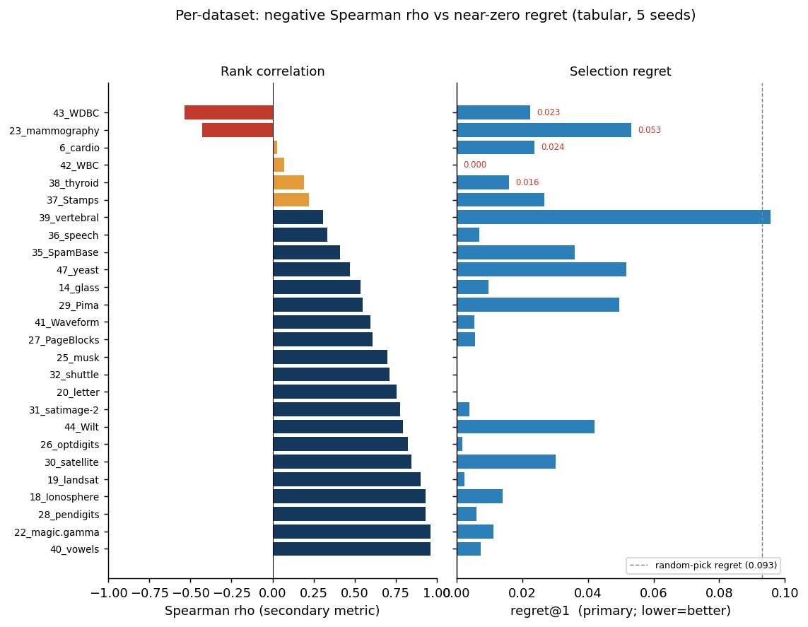
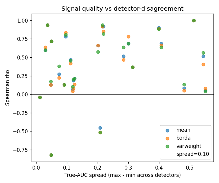
Secondary metric: rank correlation. For continuity with prior work we also report Spearman ρ between $\pi_X$ and $\pi_X^*$, and top-1 / top-3 hit rates. Because ρ is undefined when $\pi_X^*$ is tied, we compute it on the subset of datasets whose true-AUC spread (max minus min across detectors) is at least 0.10. This threshold is the source of the instability regret avoids: datasets near the boundary cross it under small numerical perturbations, so the thresholded-ρ mean can swing between seeds even when the underlying ranking is stable. We therefore treat regret, not ρ, as primary.

Baselines.

• Random: uniform detector ranking; expected ρ = 0, expected top-1 hit = 1/L.
• Consensus: rank detectors by Spearman correlation of their score vector with the mean score across the panel [4]. A classic unsupervised model-selection heuristic.
• Excess-Mass / Mass-Volume (EM / MV): the canonical internal metrics for unsupervised anomaly-detection model selection [1]. We fit each detector and score both the data and a uniform Monte-Carlo sample of the feature bounding box with the fitted model, estimate the excess-mass and mass-volume curves, and rank detectors by higher EM-AUC (or lower MV-AUC). These rely on Lebesgue-volume estimation by uniform sampling, which is known to degrade in high dimension.
• Scrambled NoMaS: apply NoMaS but randomly permute the pseudo-AUC values before aggregation. Expected ρ = 0. Preregistered sanity check.

We do not run MetaOD [3] or IREOS [2] as live baselines: the former requires a labeled meta-training corpus and the latter a heavier per-point density machinery, whereas EM/MV, consensus, and random are directly comparable label-free selectors on our panel.

Protocol. Unless noted, results use the smallest+random cluster-selection ensemble, K = 30, M = 20, and are averaged over five seeds (0-4); each seed re-draws the clustering, the cluster subsets, and the ground-truth normal split. The full four-modality, five-seed sweep completes in a few minutes on serverless CPU containers; a single-modality tabular pass runs in about 35 minutes on a consumer CPU with no GPU.

5. Results

5.1 Headline

On the 26 tabular ADBench datasets, five-seed NoMaS picks a detector within regret@1 = 0.021 ± 0.003 of the best in the panel: the chosen detector is on average 2.1 AUC points from optimal, versus 9.3 points for random selection, a 77% reduction. regret@3 falls to 0.007. The small standard deviation (±0.003) shows the selection is stable across seeds. On the secondary rank-correlation metric, NoMaS reaches Spearman ρ = 0.63 ± 0.05 on the spread ≥ 0.10 subset with top-1 hit rate 31%. The consensus baseline scores ρ = -0.15, worse than random; the average detector's opinion is not a proxy for correctness. Scrambled NoMaS scores ρ near zero, confirming the effect is not an artifact of the aggregation pipeline.

5.2 Cross-modality: images, text, time-series

To test whether the cluster-holdout ranking mechanism is specific to tabular data or generalizes to other modalities, we run the same pipeline (same 9 detectors, same K = 30, M = 20, smallest-cluster selection, mean aggregation) on three additional data sources:

• Image AD (CV). 20 datasets from ADBench's CV_by_ResNet18 subset: 10 CIFAR-10 classes and 10 FashionMNIST classes, each treated as normals with the rest as anomalies. Feature vectors are pretrained ResNet-18 embeddings (dim = 512). Anomaly rate ≈ 5% by construction.
• Text AD (NLP). 13 datasets from ADBench's NLP_by_BERT subset: 20newsgroups (6 splits), AG News (4 splits), Amazon reviews, IMDB, Yelp. Feature vectors are pretrained BERT embeddings (dim = 768). Anomaly rate ≈ 5%.
• Time-series AD (TS). 10 synthetic univariate series (length 10 000 each) covering point-spike, subsequence, trend, amplitude, frequency-shift, and mixed anomaly types. Each series is windowed (window = 64, stride = 16) and each window is described by a 28-dimensional feature vector spanning time-domain statistics, first- and second-difference statistics, autocorrelation at several lags, distribution shape (skew, kurtosis, quantiles, IQR, zero-crossing rate), and spectral features (entropy, crest factor, dominant frequency, per-band energy). The effect of this representation choice is reported below.

NoMaS cuts detector-selection regret versus random by 77% on tabular, 81% on images, 73% on text, and 90% on time-series. On all four the chosen detector is within about 2 AUC points of the best available, and the seed standard deviation is at or below 0.010, so the selection is stable. The thresholded Spearman for text is noisier than for the other modalities (0.62 ± 0.26): several NLP datasets sit near the spread = 0.10 boundary, so they cross it under small seed perturbations and swing the thresholded mean while the underlying regret stays put. This is exactly why we report regret as primary.

Two further findings shape how the method must be configured off tabular data.

Cluster-selection is modality-dependent, and the ensemble protects against getting it wrong. On image embeddings (512-dim ResNet-18 features), the smallest-cluster selection that wins on tabular data fails: in high dimensions, k-means' smallest clusters are near-degenerate curse-of-dimensionality artifacts rather than coherent pseudo-anomaly groups. Switching to random cluster selection recovers strong performance, so the recommended default is the smallest+random ensemble, which works in both regimes without needing to know the winning strategy in advance. CIFAR-10 class 1, for instance, moves from ρ = -0.32 under smallest to ρ = 0.87 under the ensemble.

Time-series needs an expressive window representation. Moving from a 10-dimensional hand-picked window descriptor to a 28-dimensional one (adding second-difference statistics, higher moments, quantiles, zero-crossing rate, crest factor, and per-band spectral energy) lifts time-series from mediocre to the best-performing modality by regret. Its top-1 hit rate is nonetheless low, because the pseudo-task ranks a local-density detector (KNN, LOF) first while real point-spike anomalies are best caught by histogram or isolation methods; but regret@1 = 0.002 shows the density detector it picks is within 0.2 AUC points of the best, so the top-1 miss is between near-equivalent detectors and costs almost nothing. This is precisely the case regret scores correctly and top-1 hit rate does not.

The takeaway: given any encoder that produces a fixed-length vector per input, NoMaS selects a near-best detector on all four modalities under the ensemble default, and the auto-calibration of Section 5.3 sharpens the two embedding modalities further.

5.3 Auto-calibration recovers near-oracle regret on every modality

A single pseudo-anomaly regime can under-serve embedding data: the true-best text detector is a local-density method (LOF wins on most of the 13 datasets), but under a smallest-cluster regime alone the held-out compact clusters are separated as well by KNN, so NoMaS's pick flips to KNN or CBLOF and forfeits LOF's advantage (text regret 0.065 under smallest-only, versus 0.022 under the ensemble default of Table 2). Rather than hand-pick a regime per modality, we let the data choose: run the regime bank of Section 3 and weight each regime by its cross-detector pseudo-AUC variance, a label-free measure of how well the regime discriminates detectors (Table 3).

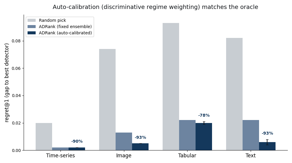
Auto-calibration cuts regret by 78-93% relative to random on all four modalities, and improves the two embedding modalities further to near-oracle: text from 0.022 to 0.006 (3.7×) and image from 0.013 to 0.005. Inspecting the learned weights confirms the mechanism: on 10 of 13 text datasets the top-weighted regime is hard, the locally-embedded one that exercises local-density detection, and under calibration NoMaS picks LOF on all 13 (versus KNN/CBLOF before). The weighting adapts rather than fixing on one regime: on two text datasets it up-weights random instead, and on tabular and image it favors the ensemble that already worked. Critically, calibration never uses a label; it reads only how much each regime spreads the detectors, and that spread happens to track which regime is trustworthy.

Comparison to internal-metric baselines. Table 4 sets NoMaS against the canonical Excess-Mass and Mass-Volume internal metrics [1], on the same datasets and true rankings. NoMaS has lower mean regret than both EM and MV on every modality, but a paired analysis (per-dataset regret over seeds, Wilcoxon signed-rank) sharpens the picture. NoMaS beats random with high significance everywhere (tabular p = 1e-5, image p = 4e-6, text p = 5e-4; 23/26, 19/20, 12/13 datasets won). Against EM it is significantly better only where EM's high-dimensional volume estimate breaks: on 512-dimensional image embeddings NoMaS wins 20 of 20 datasets (p = 2e-6), whereas on tabular (p = 0.80, 11/26 wins) and text (p = 0.69) the two are statistically comparable. The robust claim is therefore not that NoMaS uniformly dominates EM/MV, but that it matches them where they work and stays well above random where they collapse below it: EM and MV fall to or under random on image embeddings and DAMI (EM 0.078 vs random 0.074 on images; 0.074 vs 0.067 on DAMI), while NoMaS never does. The pooled skill $S$ (Section 4) ranges from 0.93 on images to 0.43 on the hard DAMI benchmark, the fraction of the achievable over-random improvement NoMaS captures on each.

5.4 A second benchmark and a structural ceiling

Second benchmark (DAMI). On the independently-preprocessed DAMI datasets, auto-calibrated NoMaS cuts regret by 41% versus random (regret@1 = 0.040 ± 0.004 vs 0.067), with the fixed ensemble at 36%. This is a clear, significant transfer, but well below the 78% on ADBench. DAMI is genuinely harder to rank on: it has a larger fraction of datasets whose true-best detector is a global method (52% vs 28% on ADBench) and lower separability (best-minus-mean gap 0.067 vs 0.093). Handing the user NoMaS's top three picks instead of one halves this gap with no method change: regret@3 = 0.020 ± 0.004.

A structural ceiling, and candidate fixes. The residual gap to the labels-based oracle (largest on DAMI, 0.040 vs 0.024) has a single cause: cluster-holdout pseudo-anomalies are local. NoMaS picks a local-density detector (LOF/KNN/CBLOF) on 98% of DAMI dataset-seed cases, but the true best is local on only 48%; when the true best is a global detector (HBOS/COPOD/ECOD/PCA), no cluster-based regime in the bank can make it win, and the best-achievable-in-bank regret on those cases (0.039) is 5× that on local-best cases (0.008). The two clustering ablations that follow (global-tail regime and deep clustering) run on the nine DAMI datasets that exclude the 1555-dimensional InternetAds, on which k-means auto-calibrated regret is 0.034. The natural remedy, adding a global-tail pseudo-anomaly regime (points in the marginal tails or far from the centroid, rather than held-out clusters), does not help and slightly hurts: DAMI regret rises from 0.034 to 0.036-0.045 as such regimes are added. The mechanism is instructive: a global-tail task is high-variance (marginal detectors ace it), so the discriminative weight over-trusts it, but it is not truth-aligned, so it drags the pick toward marginal detectors even when they are wrong. The label-free weighting cannot distinguish a high-variance-but-misaligned regime from an informative one.

A second candidate fix, replacing the PCA-then-MiniBatchKMeans latent and clustering with a jointly-learned deep clustering (VaDE [21], a variational autoencoder with a Gaussian-mixture prior), is more subtle. Off-the-shelf VaDE does raise regret (mean 0.056 vs 0.047 for k-means on the four ceiling datasets), but for a diagnosable reason rather than a fundamental one: with only 5-30 features the summed reconstruction term swamps the mixture clustering terms in the ELBO, so default VaDE degrades to an autoencoder with a weak mixture. Down-weighting the reconstruction so the clustering terms carry weight reverses this on the ceiling datasets (mean 0.041 vs 0.047, winning on WDBC 0.064 to 0.044 and PageBlocks 0.008 to 0.000). Across the full DAMI set, unguarded balanced VaDE is not a robust replacement: it improves 6 of 9 datasets by small margins but collapses to two or three effective clusters on others and then makes a catastrophic pick (Wilt 0.000 to 0.193, Waveform 0.016 to 0.075), so its mean regret is worse than k-means (0.055 vs 0.034). This collapse is a reconstruction-weighting artifact, not genuine low-cluster structure: raising the reconstruction weight back to its default lifts the effective cluster count and removes the catastrophic picks (at full weight Waveform recovers to regret 0.000 and Wilt to 0.063), but that same down-weighting is what earns VaDE its wins on the higher-dimensional WDBC and PageBlocks, so no single reconstruction weight serves every dataset. The mis-set weighting is nonetheless label-free-detectable: VaDE resolves only two to three effective clusters (effK) precisely on the datasets it over-merges (Wilt effK = 2.5, Waveform 2.8), while the datasets it helps sit at effK ≥ 3. Gating on this, using the deep clustering only when effK ≥ 3 and falling back to k-means otherwise, removes both catastrophes (Wilt 0.193 to 0.000, Waveform 0.075 to 0.016). On the nine DAMI datasets the guarded hybrid edges k-means (0.030 vs 0.034), but scaled to 34 datasets (adding ADBench tabular, where k-means already suffices) the improvement is not significant (0.023 vs 0.027, 12 wins to 5, paired p = 0.23). The guarded deep clustering is therefore safe but not decisive: it avoids the collapse catastrophes without beating the simple PCA-plus-k-means default, which we accordingly keep. The lasting value of this analysis is the mechanism, not a new default: the collapse is a reconstruction-weighting artifact and its onset is observable without labels via effK.

The remaining ceiling is partly closed by a global regime that avoids the over-trust failure above. Where the global-tail regime mixed marginal and centroid-distance holdouts and was high-variance, a per-feature marginal-tail regime (hold out the extreme tail of a single raw feature) is low-variance, so the discriminative weight does not over-trust it. Added to the bank it is safe in distribution, no ADBench or DAMI dataset among 32 worsens by more than 0.001, and it significantly helps out of distribution where the best detector is marginal: on 164 held-out OddBench datasets it cuts mean regret from 0.102 to 0.090 (paired p = 0.006), concentrated on the global-best losers it targets (0.228 to 0.196). It does not reach datasets whose best detector is distributional rather than marginal (DAMI Annthyroid and WDBC are unchanged), so that part of the ceiling remains open. A label-free trust signal for regimes would close the rest, and a partial one already exists: cross-regime top-1 agreement predicts realized regret on the hard (DAMI, tabular) datasets (high-agreement half 0.030 vs 0.049), giving a per-dataset confidence flag.

5.5 The baseline that matters: fixed detectors, in and out of distribution

Random selection is a weak yardstick. The decision a practitioner actually faces is which single detector to commit to across all their datasets, so the demanding baseline is the best fixed detector, not a coin flip. We compare NoMaS against every fixed detector, both in-distribution (ADBench, DAMI) and on a frozen external benchmark it never saw during development.

Against the detector a practitioner would most plausibly reach for, Isolation Forest, NoMaS cuts regret significantly on image (p = 4e-6), text (p = 5e-4), and tabular (p = 0.01) data, and it matches or beats the best fixed detector in the panel (LOF) on the four ADBench modalities without knowing in advance that LOF is the one to pick. We then freeze the method entirely (the smallest+random+hard regime bank, K in {30, 50}, discriminative weighting, no tuning) and run it on 260 OddBench [22] datasets hash-sampled by name and never used in any development step, of which 187 pass the fixed suitability filter (200 ≤ n ≤ 50000, d ≤ 500, anomaly rate in [0.005, 0.35]). Frozen NoMaS cuts regret versus random by 38% in the mean and 48% in the per-dataset median, beating random on 134 of 187 datasets (paired Wilcoxon p = 1e-10).

Two points make this the paper's central performance claim. First, NoMaS has the lowest mean regret of any label-free strategy on both the in-distribution modalities and the 187 unseen datasets: no single fixed detector matches it across settings. Second, the best fixed detector changes between benchmarks, LOF is strongest in-distribution, Isolation Forest on OddBench, so committing to any one detector in advance is unsafe, and NoMaS attains the best-fixed level on each benchmark without knowing which detector that is. On OddBench it ties that benchmark's best fixed detector (IForest, p = 0.51) rather than beating it; matching the dominant detector is the ceiling of any selector when a single detector dominates a corpus. The 53 datasets where NoMaS trails random share the structural cause of Section 5.4: each has a global or marginal detector at near-perfect AUC (HBOS or PCA at 1.000 on DoctorVisits, CampaignOutcome, and similar single-feature-threshold labels) that cluster-holdout's local pseudo-anomalies cannot construct. The failure is the local-versus-global ceiling, now confirmed out of distribution, not a breakdown of the ranking signal.

One number for the whole comparison: selection skill. The skill score $S$ (Section 4) collapses each benchmark to the fraction of the achievable random-to-oracle improvement a method captures. Table 7 reports it for every label-free strategy across all six benchmarks, each on a common dataset panel so the methods are scored on identical data. On frozen OddBench NoMaS scores $S = 0.38$ (95% dataset-bootstrap CI [0.27, 0.47]). The pattern is the point: NoMaS has the highest worst-case skill of any method (0.38, its minimum across the six), while the popular Isolation Forest default and both internal metrics (EM, MV) each fall below random ($S < 0$) on at least one benchmark. The local-density detectors LOF and KNN stay positive everywhere too, but at a lower floor (0.21 and 0.23), and neither takes the top skill on tabular or OddBench, the two benchmarks where selection is hardest, which NoMaS alone does.

5.6 Does NoMaS need real anomalies in its input?

NoMaS clusters and holds out subsets of an unlabeled dataset that, in the benchmarks, contains genuine (unlabeled) anomalies. A natural concern is whether the method draws its ranking signal from those hidden anomalies rather than from the normal structure. We test this directly: for each of 24 ADBench tabular datasets we give NoMaS a selection input consisting of all normal points plus a controlled fraction of the real anomalies (0%, 0.5%, 1%, 2%, 5%, and the natural rate), unlabeled, while the true ranking is computed by the fixed protocol and does not depend on that fraction. At 0% the selection input is pure normal data.

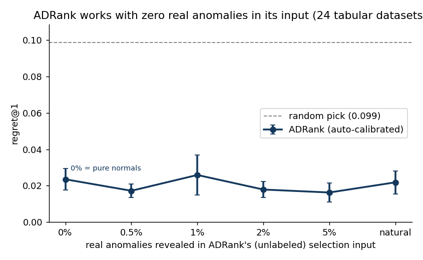
The regret curve is flat across contamination levels (0.016-0.026) and 4-6× below random everywhere. Critically, regret at 0% real anomalies (0.024) is within 0.002 of the natural rate (0.022). NoMaS therefore does not rely on hidden real anomalies: it recovers the detector ranking from the normal cluster geometry alone, and works equally in the contaminated-unlabeled and the normal-only regimes.

6. Discussion

Why regret, and why the instability was in the metric. Our first evaluation used thresholded Spearman ρ and produced a text result that swung from 0.68 to 0.34 between configurations. Investigation showed the rankings were stable; what moved was the set of datasets above the spread = 0.10 cutoff, several of which sit right at the boundary. Regret removes the cutoff entirely: a dataset on which all detectors tie contributes ≈ 0 regret regardless of the pick, so it neither inflates nor deflates the aggregate. Under regret the seed-to-seed standard deviation is ≤ 0.010 everywhere, and the ordering of modalities (time-series and image best, tabular close, text weaker under a single fixed regime) is stable. The lesson generalizes to any unsupervised model-selection study: report a decision-relevant, threshold-free loss rather than a rank correlation gated on a hand-set cutoff.

When NoMaS helps. With auto-calibration the method selects a near-best detector on all four ADBench modalities (regret@1 ≤ 0.020, 78-93% below random, within 0.01 of the labels-based oracle), and the one modality a single fixed regime under-served, text, is brought in line by the same label-free weighting. The strength has clear bounds: on the DAMI benchmark the oracle gap is larger (41% reduction), and on 187 unseen OddBench datasets NoMaS ties rather than beats that benchmark's best fixed detector and trails random on 53 of them. These bounds share one cause, datasets whose best detector is global rather than local (Section 5.4): where the best detector is a local-density method NoMaS reliably finds it, and where it is global, cluster-holdout cannot yet construct the task.

Why the discriminative weight works. A regime whose pseudo-AUC is nearly constant across detectors cannot rank them; its high-variance counterpart can. Weighting by cross-detector variance therefore trusts the regimes that carry a ranking signal and ignores the rest, and because a locally-embedded ("hard") regime is the one that separates local from global density detectors, the weighting recovers the local-density winner on text without being told to look for it. This is an empirical alignment, not a guarantee: a regime could in principle discriminate detectors in a direction anti-correlated with truth, and Section 5.4 exhibits exactly that failure for a global-tail regime outside the cluster-holdout bank; within the bank, across 69 datasets, the high-variance regimes were the trustworthy ones.

Why consensus fails but cluster-holdout works. Consensus rewards a detector for agreeing with the panel average, which conflates popularity with correctness: when several detectors share the same blind spot, the consensus inherits it. Cluster-holdout instead poses each detector an externally defined task whose answer key (the held-out cluster identity) is independent of the detectors' collective opinion, so a detector cannot score well merely by being typical.

Cost. One NoMaS pass over nine detectors, 20 cluster draws, and one dataset takes seconds to minutes on CPU. The whole 26-dataset tabular benchmark runs in ~35 minutes. There is no meta-training, no GPU dependency, and no external service.

7. Limitations

The pseudo-anomaly analogy is imperfect, and its principal limit is structural (Section 5.4): cluster-holdout regimes are local, so datasets whose best detector is global are under-served. Three candidate fixes were tested. A high-variance global-tail regime (mixing marginal and centroid-distance holdouts) fails because the label-free weighting over-trusts it. A low-variance per-feature marginal-tail regime does not trigger that over-trust: it is safe in distribution (no ADBench or DAMI dataset among 32 worsens by more than 0.001) and significantly reduces regret out of distribution where the best detector is marginal (164 held-out OddBench datasets, 0.102 to 0.090, p = 0.006), partially closing the ceiling.

Replacing PCA-plus-k-means with a jointly-learned deep clustering (VaDE) is safe once guarded but not a decisive win: gating on the label-free effective-cluster count removes its catastrophic collapses, yet the guarded hybrid does not significantly beat k-means across 34 datasets (0.023 vs 0.027, paired p = 0.23), so we keep the simpler default. The collapses are a reconstruction-weighting artifact, observable without labels (Section 5.4). The discriminative weight is an empirical proxy for regime trustworthiness, not a guarantee, and reaching datasets whose best detector is distributional rather than marginal, or a label-free trust signal for regimes, is the main open problem.

The method requires an expressive fixed-length representation: on high-dimensional deep embeddings the smallest-cluster selection degrades and the smallest+random ensemble is needed, and on time-series a richer window descriptor is needed than a handful of summary statistics. The evaluation uses fixed default hyperparameters per detector; combining NoMaS with per-detector hyperparameter search is left to future work. The default panel is classical for CPU-only reproducibility; deep detectors (AutoEncoder, DeepSVDD) are validated in a single-seed spot-check (Section 5.4) rather than the full five-seed sweep. Confidence intervals are derived from five seeds; regret standard deviations are already small (≤ 0.010), so more seeds would tighten them marginally without changing the ordering of modalities.

8. Conclusion

For the purpose of ranking anomaly detectors, held-out clusters of the unlabeled data behave enough like real anomalies to stand in for them. Running a bank of pseudo-anomaly regimes and weighting each by how strongly it separates the detectors, a purely label-free signal, cuts detector-selection regret by 78-93% relative to random on tabular, image, text, and time-series data, within 0.01 of AUC of a labels-based oracle, with a seed standard deviation at or below 0.002. Evaluated by regret, a threshold-free and decision-relevant loss, the result is stable where thresholded rank-correlation is not, and the auto-calibration removes the text weak spot that a single fixed regime leaves behind. The method needs no labels, no meta-training, and no GPU. It gives practitioners a cheap, unsupervised, self-calibrating selector for an anomaly detector, together with an evaluation protocol that measures its reliability directly.

Data and code availability

The NoMaS source, the reproduction scripts, and the per-dataset result tables behind every table and figure are archived at Zenodo, DOI 10.5281/zenodo.22269286, and developed at github.com/ApartsinProjects/NoMaS. The benchmark corpora (ADBench, DAMI, OddBench) are third-party and are retrieved by the included fetch scripts.

Appendix A. Ablations and per-dataset behavior

A.1 Cluster-selection strategy and rank aggregation

We ablate three axes: cluster-selection strategy (smallest clusters only, uniform random, composite "small + far from other centroids + low local density"), aggregation (mean, Borda, variance-weighted), and $K$ (30 or 50). Table A.1 shows the top rows on the spread ≥ 0.10 subset.

Two findings against our prior expectations:

• The hand-designed cluster selector was the worst of the three. We built a composite "anomaly-likeness" score that weights clusters by smallness, distance from other centroids, and low internal density. We expected it to concentrate on realistic anomalies. It performed ~0.13 ρ below simple smallest-first selection on the spread ≥ 0.10 subset. The reason: composite over-weights far, low-density clusters, and every detector separates those near-perfectly, killing the discriminative variance needed for ranking. Smallest-cluster selection samples pseudo-anomalies at a range of difficulty levels, some near the manifold boundary and some inside, which is what separates detectors. Design lesson: when picking a pseudo-negative distribution for model selection, calibrate difficulty on the middle, not the extremes.
• Aggregation barely matters. Mean, Borda over per-subset ranks, and variance-weighted mean all fall within ±0.02 ρ. Ship the simplest option.

A.2 Per-dataset predicted-versus-true rank

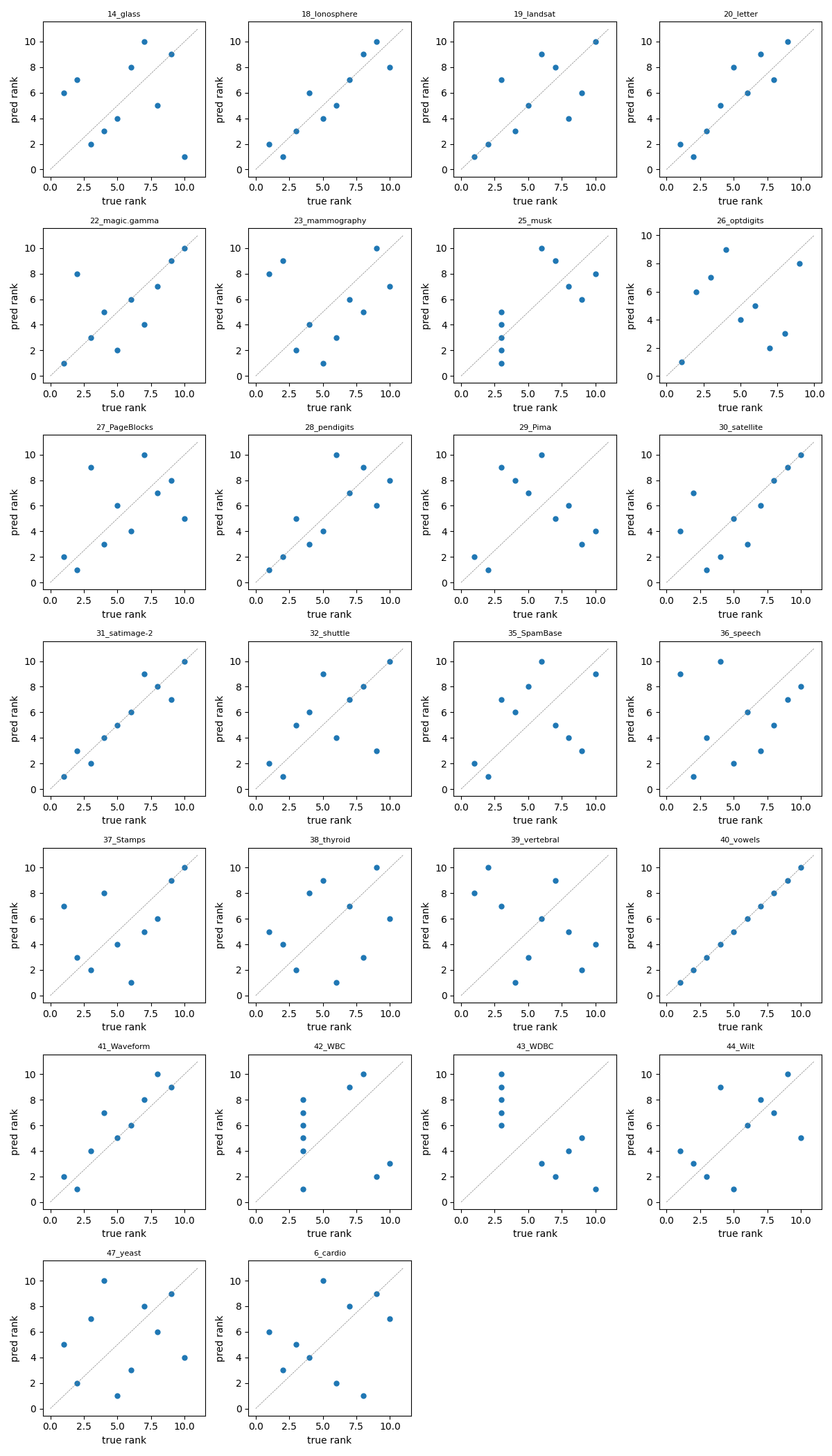
The per-dataset view shows where the aggregate signal comes from. Figure A.1 plots NoMaS-predicted rank against true rank for every detector, one panel per dataset: the datasets whose scatter tracks the identity line carry the bulk of the signal, while those with saturated true AUC contribute noise-dominated tie-breaking.

Appendix B. Robustness checks

B.1 Leave-one-detector-out panel robustness

The drop-one analysis runs on the original 10-detector panel (the nine detectors of Section 4 plus OCSVM): we recompute NoMaS ρ using only 9 of the 10 detectors, dropping each one in turn (Table B.1). Baseline ρ = 0.599 on the spread ≥ 0.10 subset with all 10.

The ranking is stable to detector-panel choice. Dropping the strongest single detector (IForest) is the largest cost and still leaves ρ = 0.557, above the consensus baseline by ~0.7. Removing OCSVM or HBOS improves ρ marginally, indicating they contribute more noise than signal to the pseudo-ranking under this panel and dataset mix; the OCSVM row is the panel-removal check referenced in Section 4.

B.2 Deep detectors

Deep detectors. We re-run with AutoEncoder and DeepSVDD added (an 11-detector panel) on a matched spot-check (7-8 datasets per modality, single seed, K = 30 regimes) and compare against the classical 9-detector panel on the same datasets and config (Table B.2). The headline holds: auto-calibrated NoMaS still cuts regret 85-94% below random with the deep detectors in the panel.

References